

Being able to calculate percentages is something that is very useful in spreadsheets, and is a very useful mathematical skill to have in general. When working with data in spreadsheets there will be a lot of situations where you will want to calculate the percentage of a given number relative to the total.
To calculate the percentage of a total, simply divide the part by the total (Part / Total). Sometimes the total is given in your data, and sometimes you will need to calculate it. In this lesson I will show you how to handle both scenarios.
To calculate the percentage of a number in Google Sheets, follow these steps:
- Type an equals sign (=)
- Type the number or the cell that contains the number that represents the part of the total
- Type a forward slash (/)
- Type the number or the cell that contains the number that represents the total
- Press “Enter” on the keyboard. The final formula will look like this, where the part: =25/100 (Or like this: =B2/A2)
- Click the "Format as percent" button on the top toolbar (%)
After following these steps, the formula will display the percentage that the part / portion represents when compared to the total.
This article focuses on calculating the percentage of a total / number… but if you want you can click here to learn how to calculate the percentage increase from one number to another.
Calculate percentage of a number (basic example)
Let's go over a basic example of calculating percentage. What we want to do is find the percentage that the number in cell B2 represents (the part of the whole / total), when compared to the total in cell A2.
Cell B2 contains the "Part" (25), and cell A2 contains the total (100). So the question is what percentage is 25 out of 100. To do this we divide the part by the total, which in this case is 25/100, or B2/A2 considering the cell references.
=B2/A2
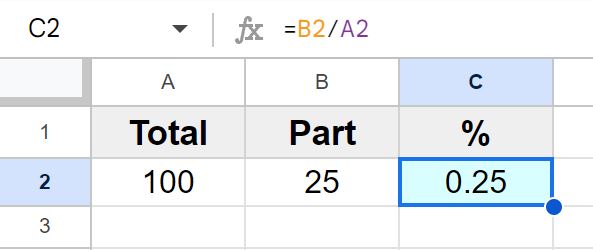
After dividing cell B2 (25) by cell A2 (100), cell C2 now displays the number 0.25.
The number 0.25 is equivalent to 25%, but now we want to make the cell actually display in percentage format.
To do this, select cell C2, then click the "Format as percent” button on the top toolbar, which has a percentage symbol on it (%).
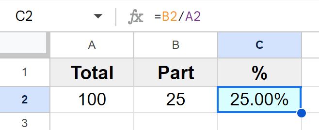
As you can see in the image above, after formatting the cell as "Percent", cell C2 now displays 25.00%. By default when you select the percentage format, Google sheets will display two decimal places.
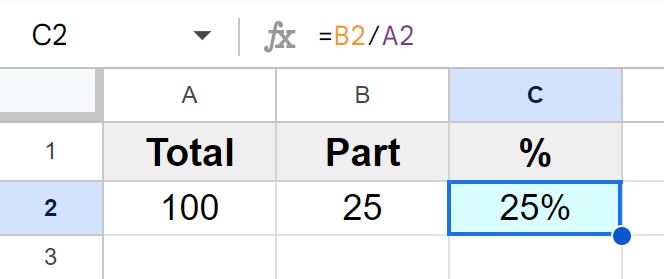
If you want to remove the decimal places, click the “Decrease decimal places" button on the top toolbar two times, and the percentage will display without decimal places like in the image below (25%).
Calculating percentage of a total (using the SUM function)
Now let's go over an example where the "Total" is not simply given in the data, and where we need to calculate the total in order to calculate the percentage.
In this example, we will use the SUM function to calculate the total by putting the SUM function in its own cell, and then refer to that cell in the division formula that calculates percentage.
What we have is data that shows how many people voted "Yes" (cell B2), and how many people voted "No" (cell B3). We will calculate the total number of people who voted for either option by using the SUM function in cell E1. Then we will calculate the percentage of people who voted “Yes" (B2/E1), and we will also calculate the percentage of people who voted "No" (B3/E1).
Cell E1
=SUM(B2:B3)
Cell C2:
=B2/E$1
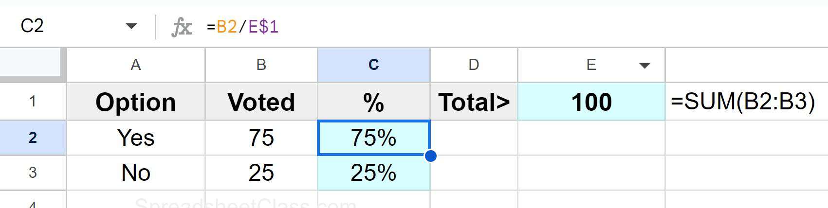
As you can see in the image above, 75 people voted "Yes", and 25 people voted "No". Cell E1 is calculating the total number of people who voted, which is 100. Cell C2 is dividing 75 by 100 (B2/E1), which yields an answer of 75%.
The formula in cell C2 was copied and pasted into cell C3, which calculates the percentage of people who voted no, which is 25% (25/100 or B3/E1)
Notice that in the formula in the example, a dollar sign was added before the row reference for cell E1, like this: E$1
This is so that the division formula could be copied down the column without adjusting the row reference for cell E1. In other words, when we copy the formula down, we do not want Google Sheets to change the reference to cell E1, because we want to keep referring to the total in cell E1 as the formula is copied down column. This is done by adding a dollar sign before the reference that we do not want to change when the formula is copied.
After the formula is copied into cell C3, the formula becomes =B3/E$1
Using the SUM function directly in the division formula
If you want, instead of designating an individual cell to use the SUM function, you can enter the SUM function directly into the division formula that calculates percentage. So just like in the previous examples, we divide by the total, but the total is calculated by the SUM function, so we are dividing by the SUM function, as shown in the image below.
So in this example the SUM function is adding up the total number of people who voted, and then we are dividing the "Part" by the total / SUM function (i.e. people who voted "Yes" divided by the total number of people who voted, and people who voted "No" divided by the total number of people that voted).
=B2/(SUM(B$2:B$3))
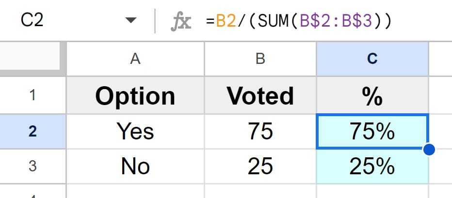
As you can see in the image above, just like in the last example, cell C2 shows that 75% people voted "Yes", and cell C3 shows that 25% people voted "No". In this case we did it by using one single formula, with the SUM function entered directly on the bottom of the division formula..
Especially since this example only had two different items that compose the total, we could have also used basic addition instead of the SUM function to get the total, as shown in the formula below.
=B2/(B$2+B$3)
Calculating percentage of multiple test scores
Now let's go over an example using more rows of data. In this example we are going to calculate the percent that each student scored on a test, given the score and the total possible points for the test.
To calculate the percentage score in a Google spreadsheet, type an equal sign, then type the score that was earned or the cell that contains this score, type a forward slash (/), then type the number that represents the total possible points or the cell address that contains that number. Press "Enter" on the keyboard.
As shown below, column B contains the total possible points for each test/student, which in this case is the same for each test. Column C contains the score that each student attained on the test. Column D will contain our formulas that calculate the percentage score for each student.
We simply divide the score by the points possible, (Score / Possible) which in this case is cell C2 divided by cell B2 (=C2/B2).
=C2/B2
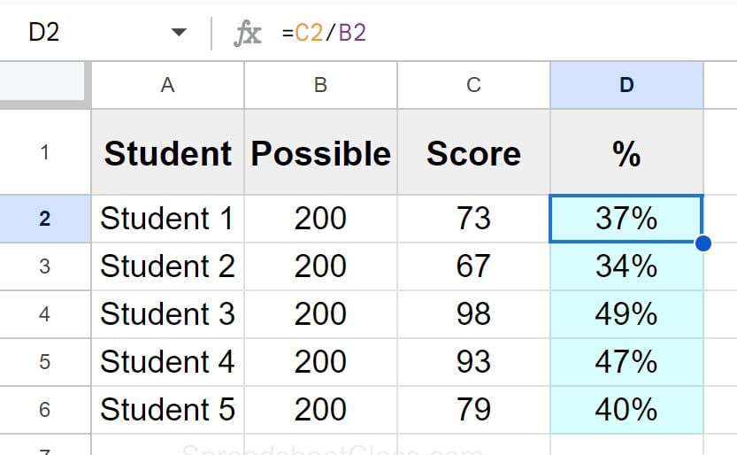
As you can see in the image above, cell D2 displays 37%, which is 73 (points earned) divided by 200 (points possible). The formula has been copied down the column to calculate the percentage for each student.
Although in this case the total points possible was the same for each entry/row, the formula is set up in a way that does not require the total possible points to be consistent for each row.
An example of when this comes in handy is when you have a variety of items to calculate the percentage of, where there is a different total for each entry (such as in a gradebook where each assignment has its own total points possible).
If we modified this example to be like the previous example where the total was listed at the top in cell E1, we would simply change our formula so that it divides cell C2 by cell E1, making sure to include the dollar sign in the reference to cell E1 to prevent Google Sheets from changing the reference when the formula is copied, like this: =C2/E$1.