

Sometimes you may find that you want to create a series of numbers very quickly when creating a spreadsheet, without having to manually type each number in the cells, and this can be done by using autofill, which is also sometimes simply known as “fill”.
To automatically create a series in Google Sheets, do the following:
- Type the beginning values of your series into two adjacent cells (for example the numbers 1 and 2), and highlight the cells with these values
- Click and hold the fill handle (small square at the bottom right of a highlighted cell)
- Then drag the fill handle down until you have reached the end of your series, and release your mouse click
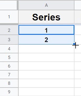
In this picture you can see that when your cursor is hovered over the small blue square at the bottom right of a cell selection, the cursor turns into a cross / plus sign, and this is what is called the “fill handle”.
When using autofill and dragging the fill handle downwards to fill values through a column/vertical range, this is referred to as “fill down”.
When using autofill and dragging the fill handle to the right to fill values through a row/horizontal range, this is referred to as “fill right”.
In some cases you can hold the “ctrl” key on the keyboard while dragging the fill handle, which will only require you to highlight the first value in the series (because doing this tells Google Sheets that you specifically want to use a series).
However, there are some cases where holding “ctrl” will not work when trying to fill a series. In many cases instead of holding the “ctrl” key, you’ll need to type the first AND second value in the series (as described above) to show Google Sheets what you intend your series to be.
This is why I will not be using the method that uses the “ctrl” button in this article, because it only works sometimes… where selecting the first two values of a series to use autofill, almost always works.
Note that with any series that can be created vertically… you can also create the same series horizontally by clicking and dragging the fill handle right instead of downward. We will go over this briefly in this article but for the most part we will stick to creating vertical lists.
You can also use autofill to copy formulas quickly, which we will also go over briefly in this article.
Below, I will show you how to create a series of numbers, dates, and other values as well, in a variety of ways by using autofill.
This article focuses on using autofill to create a series in Google Sheets, but if you want you can learn how to use autofill to create a series in Microsoft Excel.
The Google Sheets autofill / fill down shortcut
Shortcut 1 (Double clicking the fill handle):
There is a really great shortcut that you can use to autofill without dragging, which works in many cases when you are creating a series.
If you double click the fill handle when there is adjacent data to the series you want to create, it will automatically fill down the series to the bottom of the data that is adjacent to your formula/series.
Shortcut 2 (ctrl+D):
The keyboard shortcut “Ctrl” + “D” will copy/fill the contents of the cell at the top of the selected range, through the entire selected range. This works very well to copy down the formulas through a selected range… but for creating a series of values this shortcut does not always work for every type of list/series.
The same applies for the fill right shortcut, which is “Ctrl” + “R”.
How to create a numbered list with autofill in Google Sheets
Let’s start by going over the different ways that you can automatically create a list of numbers in Google Sheets.
Create a series that increments by 1
First let’s create a numbered list, which is the most common task when creating a series with “fill down”.
To automatically create a list of numbers, do the following:
- Start by typing the number 1 into cell A2, and then typing the number 2 into cell A3
- Highlight the cells A2 and A3, then click (and hold) the fill handle
- Then while still holding your mouse click, drag your cursor downwards until you have reached cell A12
- Release the mouse click, and your series of numbers will appear
Create a series with a pattern
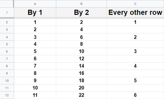
You can also create a series based on a pattern in Google Sheets, such as a list of numbers that increments by 2, or by 10.
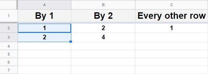
To create a series of numbers that increments by 2 each time, begin your series with the numbers 1 and 3, as shown in the example image above in column B.
Number every other row
To create a series of numbers that skips every other row, begin your series with the number 1 followed by a blank cell beneath it, as shown in the example above in column B.
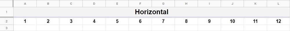
How to create a horizontal numbered list
You can also create a series horizontally by using “fill right”, and dragging the fill handle right instead of downwards.
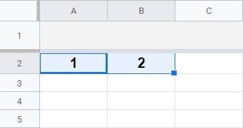
In this example we will create a series of numbers that increments horizontally to the right.
To do this, type the number 1 into the cell A2, and then type the number 2 into the cell B2.
Then highlight cells A2 and cell B2.
Now click, hold, and drag the fill handle to the right, until you have reached cell L2.
Release your mouse click, and a horizontal series of numbers will appear.
Using the ROW and COLUMN functions to create numbered lists
Another way to easily create a list of numbers in Google Sheets, (specifically a series that is attached to the row/column number), is by using the ROW and COLUMN functions.
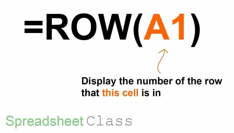
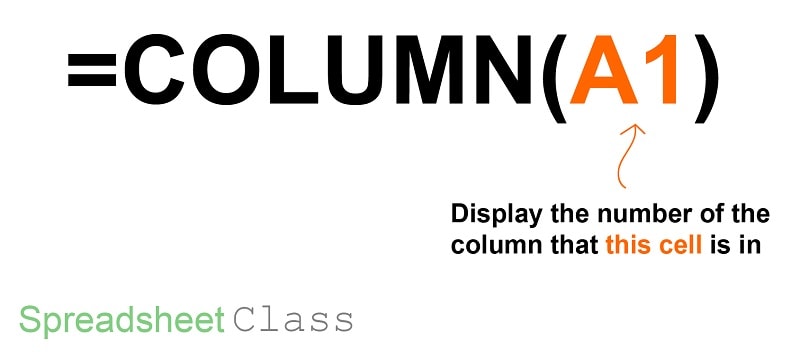
The ROW function will tell you the number of a row when given a cell reference, and the COLUMN function will tell you the number of a column when given a cell reference.
ROW function diagram:
The Google Sheets ROW function description:
Syntax:
ROW([cell_reference])Formula summary: “Returns the row number of a specified cell.”
COLUMN function diagram:
The Google Sheets COLUMN function description:
Syntax:
COLUMN([cell_reference])Formula summary: “Returns the column number of a specified cell, with A=1.”
Creating a numbered list with the ROW function in Google Sheets
Below I have shown two different ways that you can apply the row function to create a series of numbers.
The first way is by entering the ROW formula in the first cell, and then filling down the formula so that there is a formula in each cell (Google Sheets will automatically adjust the cell reference).
The second way is by using the ARRAYFORMULA function to apply the ROW formula to the entire range/column with a single formula.
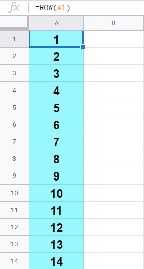
How to use autofill with the ROW function
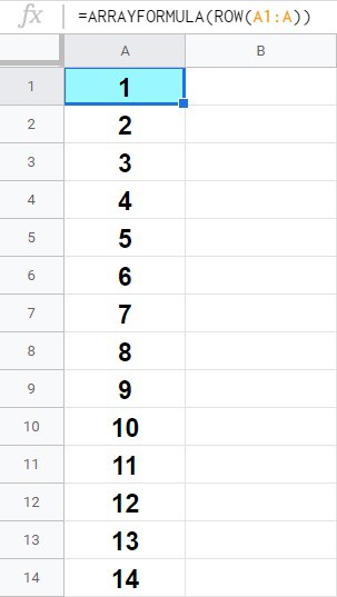
To enter a ROW formula into each cell of a column/ vertical range, enter the formula below into cell A1, then click and drag the fill handle down until you reach cell A14.
Release the mouse click and a series of numbers will have appeared (because the row function is copied/filled to each cell).
Formula: The formula below is entered into the blue cell (A1), for this example
=ROW(A1)
Using the ARRAYFORMULA function with the ROW function
The other way to apply the ROW function to multiple cells, is by using the ARRAYFORMULA function. This will allow you to have one formula that applies itself to the cells below as if there were individual ROW formulas in each cell.
To use the ARRAYFORMULA and ROW functions as shown in the example below, enter the formula below into cell A1.
Your series of numbers will appear just like in the last example, but this time with only using one formula.
Formula: The formula below is entered into the blue cell (A1), for this example
=ARRAYFORMULA(ROW(A1:A))
Creating a horizontally numbered list with the COLUMN function in Google Sheets
The same type of logic from the last examples can be used to create a horizontal series of numbers, by using the COLUMN function.
How to use autofill with the COLUMN function
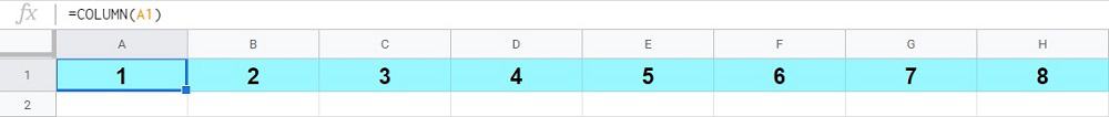
To enter a COLUMN formula into each cell of a row/ horizontal range, enter the formula below into cell A1, then click and drag the fill handle right until you reach cell H1.
Release the mouse click and a series of numbers will have appeared (because the COLUMN function is copied/filled to each cell).
Formula: The formula below is entered into the blue cell (A1), for this example
=COLUMN(A1)
Using the ARRAYFORMULA function with the COLUMN function
The other way to apply the COLUMN function to multiple cells, is by using the ARRAYFORMULA function. This will allow you to have one formula that applies itself to the cells to the right, as if there were individual COLUMN formulas in each cell.
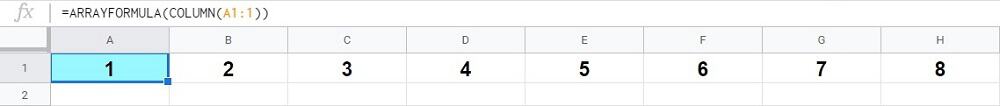
To use the ARRAYFORMULA and COLUMN functions as shown in the example below, enter the formula below into cell A1.
Your series of numbers will appear just like in the last examples, but this time with only using one formula.
Formula: The formula below is entered into the blue cell (A1), for this example
=ARRAYFORMULA(COLUMN(A1:1))
How to autofill a sequence of dates in Google Sheets
There are several ways that a sequence of dates can be created with autofill, by using the same process that was described for creating a series of numbers.
Below is an example that shows multiple ways to fill in dates. In the first image you can see the first two values in each series, and the second picture will show the full series that each will create after clicking and dragging the fill handle.
In this example we will stick to creating a vertical series, but note that any of these methods for filling dates can also be used horizontally if you simply drag the fill handle right instead of down.
For each type of date sequence below, follow the instructions below, after entering the first two values of the series indicated in each section.
- To automatically create a sequence of dates, after typing the first two dates in the series that you want to create… highlight the first two values/cells in the series, then click (and hold) the fill handle
- Then while still holding your mouse click, drag your cursor downwards until you have reached the cell where you want your series to end
- Release the mouse click, and your sequence of dates will appear
Create a sequence of dates that increments by day
To create a date sequence that increments by day, begin your series with the date of the first day in the sequence, and then also enter the date of the following day, in the cell below it.
Here are the first two days used for the series in the example shown below, in column A:
1/1/2019
1/2/2019
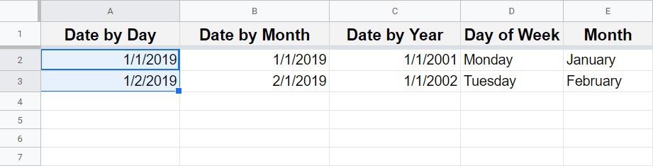
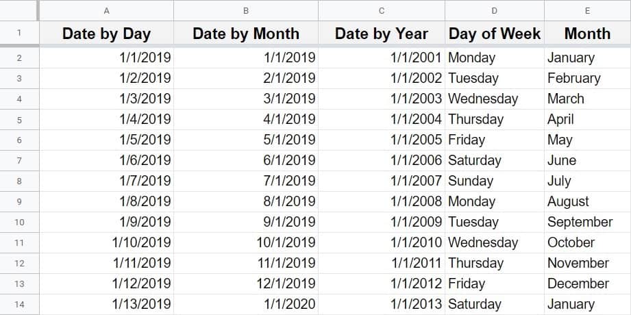
Create a sequence of dates that increments by month
To create a date series that increments by months, begin your series with the date of the first month in the sequence, and then also enter the date of the following month, in the cell below it.
Here are the first two months used for the series in the example shown above, in column B:
1/1/2019
2/1/2019
Create a sequence of dates that increments by year
To create a date sequence that increments by years, begin your series with the date of the first year in the sequence, and then also enter the date of the following year, in the cell below it.
Here are the first two years used for the series in the example shown above, in column C:
1/1/2001
1/1/20002
How to autofill text in Google Sheets
There are also some cases where you can use autofill to fill text in Google Sheets, such as by listing the days of the week, or the months of the year.
In columns D and E in the example picture above, you can see an example of using autofill with text.
List the days of the week
You can use autofill to quickly list the days of the week in Google Sheets, by beginning your series with two consecutive days of the week, such as Monday and Tuesday, as shown in the example above in column D.
List the months of the year
Just like with listing the days of the week… you can also use autofill to quickly list the months of the year in Google Sheets, by beginning your series with two consecutive months of the year, such as January and February, as shown in the example above in column E.
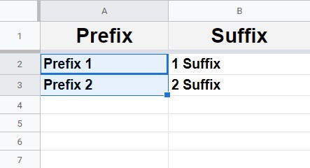
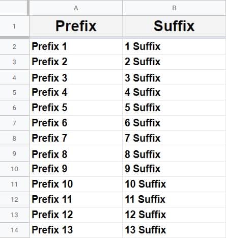
How to increment a series of values that have a prefix or a suffix
Google Sheets will also increment strings of values in a series that have a consistent prefix or suffix.
In the example shown below, I have created two different lists with autofill.
The first list (in column A) was created by beginning the series with the following two values which have the same prefix, and then dragging the fill handle down:
Prefix 1
Prefix 2
The first list (in column B) was created by beginning the series with the following two values which have the same suffix, and then dragging the fill handle down:
1 Suffix
2 Suffix
How I use autofill in my work
I am constantly using this feature in my work, especially when I need to make a list of dates, such as a horizontal list of dates for attendance trackers.
I also find myself using autofill frequently to create vertical numbered lists, such as when I have headers in my spreadsheet and want to know which entry something is in my data since using the row number will be slightly skewed by the headers.