

In this tutorial, I am going to teach you how to use Google Sheets from the ground up. You will learn all of the important things that you need to know to work with Google Sheets in the professional world, from how to create and format sheet, to using formulas and performing mathematical operations.
This lesson will get you up to speed on a lot of really important Google Sheets concepts, that you should know if you are going to be working in Google Sheets often.
Throughout the tutorial, you will find links to more in-depth lessons for some of the important topics, so feel free to expand your knowledge on these subjects and formulas.
After completing this beginner’s course, take your skills to the next level with the free dashboards and data analytics course.
And don’t forget to get your free Google Sheets cheat sheet
You may also be interested in learning the most essential formulas in Google Sheets. Check out this template / tutorial on using the best formulas in Google Sheets.
Below you will find a table of contents that shows everything that you will learn in this article / video. Timestamps are also included so that you can easily navigate through the video. These concepts are taught while building a single spreadsheet that displays test grades, and so you can simply follow along to learn each concept.
Table of contents for the VIDEO tutorial
0:00 Introduction / Creating a new sheet
1:13 About cells, cell addresses, rows, columns
2:03 Selecting multiple cells i.e. “Ranges”
2:37 Typing ranges and references
3:04 Navigating through the cells
3:34 Selecting rows and columns
5:30 Selecting non-adjacent cells, rows, and columns
6:10 Adjusting column width and row height
7:46 Adjusting multiple columns or rows at once
8:57 Entering text and numbers (Values) into cells
11:09 Cell formatting: Fill color, text color, font size, font style, alignment, wrap
13:04 Autofit column width (Automatically adjust width)
15:20 Copying and pasting cells (Without formulas)
16:47 Entering formulas (Division)
17:30 Changing the format of the cell values (Percentage)
18:05 Copying and pasting formulas
19:18 Using autofill / fill down to copy formulas
20:19 Fill right
21:29 Deleting cell contents
22:19 Freezing rows and columns
23:29 Adding new rows and columns
24:36 Deleting columns and rows
25:08 Absolute and relative cell references (Locking references)
27:37 Mathematical operators (Addition, subtraction, multiplication, division)
28:14 Quick selection shortcuts, and fill down / fill right shortcuts
30:01 Using ARRAYFORMULA to extend formulas
31:43 Cell references (Referring to a single cell)
32:30 Adding new tabs
32:47 Referring to cells from another sheet
33:30 Renaming tabs
34:29 Copying formatting with “Paint Format”
35:05 Referring to an entire column with a single formula
36:17 Moving cells, rows, and columns
38:08 The 3 cursor positions (Select, move, and fill)
39:08 Cutting cells, rows, and columns
40:05 Duplicating tabs
40:31 Deleting tabs
40:58 Using the IF function (If / Then statement)
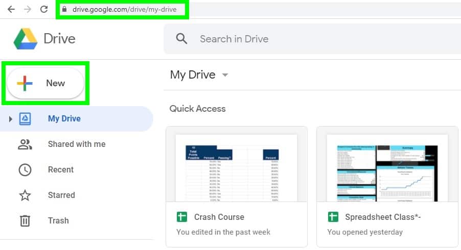
How to create a new blank Google spreadsheet
To create a new, blank Google spreadsheet, follow these steps:
- Login to your Google / Gmail account
- Go to drive.google.com
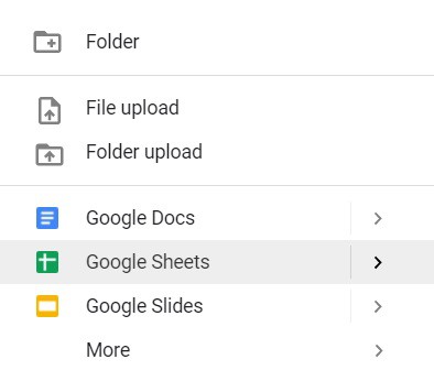
- Click the big button on the top left that says “New”
- Click “Google Sheets
By following the steps above, a blank Google spreadsheet will open. Change the name of the sheet or edit any of the cells to save the spreadsheet in your Google Drive.
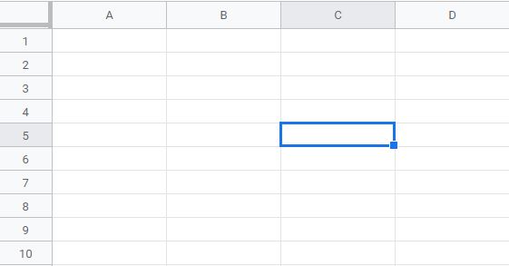
About cells, cell addresses, rows, columns
Every cell in a spreadsheet has an address. With a cell address the column is stated first, and then the row. For example, cell C5 is in column C, and in row 5.
To select a cell, click your mouse one time on the cell that you would like to select.
You must select a cell before you enter text or numbers into it, or before you change the formatting of that cell.
Select multiple cells i.e. “Ranges”
You can also select multiple cells at once in a Google spreadsheet, or in other words you can select a range of cells.
To select a range of cells, follow these steps:
- Click once in the middle of the cell that is at the top left of the range that you would like to select, and hold your click
- Drag your cursor right, downwards, or both, and then release your click when you have highlighted all of the cells that you want to select
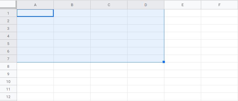
Type / notate ranges and references
To use formulas, you will need to know how to type references to cell ranges.
To type the reference to a range of cells, type the reference of the first cell (at the top left of the range), then type a colon “:”, and then type the reference of the last cell (at the bottom right of the range).
For example, if you wanted to notate the range of cells that spans from cell A1, to cell D7, you would type A1:D7.

This reference can be read as “A1 through D7″.
Navigate through the cells
There are multiple ways that you can navigate to the cell that you want to select in your Google spreadsheet.
To navigate through the cells, do either of the following:
- Click once on the cell that you want to select, and use the vertical and horizontal scroll options to access the desired cell if needed)
- Or use the arrow keys on the keyboard to move from cell to cell in the direction that you specify.
Select rows and columns
In addition to being able to select cells and ranges of cells, you can also select entire columns or rows in a Google spreadsheet.
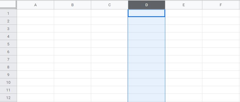
Select a column
To select a column, click on the top of the column that you want to select, on the letter that represents which column that it is, and you will have selected the entire column and all of the cells within it.
Select a row
To select a row, click on the left of the row that you want to select, on the number that represents which row that it is, and you will have selected the entire row and all of the cells within it.
Select multiple columns
To select multiple columns at once, click at the top of the first column that you want to select, hold your click, drag your cursor to the right, and release your click when you have selected all of the desired columns.
Select multiple rows
To select multiple rows at once, click at the left of the first row that you want to select, hold your click, drag your cursor downwards, and release your click when you have selected all of the desired rows.
Select non-adjacent cells, rows, and columns
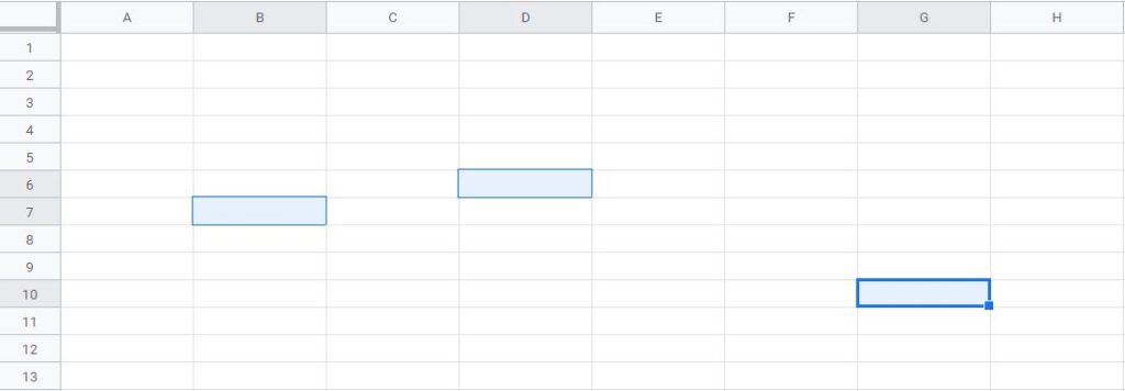
You can also select multiple cells that are not right next to each other in Google Sheets.
Select non-adjacent cells
To select non-adjacent cells, click once on the first cell that you want to select, then hold “Ctrl” on the keyboard, and then click on the other cells that you want to select.
You can do this same thing with rows and columns.
Select non-adjacent columns
To select non-adjacent columns, click once on the first column that you want to select, then hold “Ctrl” on the keyboard, and then click on the other columns that you would like to select.
Select non-adjacent rows
To select non-adjacent rows, click once on the first row that you want to select, then hold “Ctrl” on the keyboard, and then click on the other rows that you would like to select.
Adjust column width and row height
You can easily adjust the width of columns, and the change the height of rows in your spreadsheet.
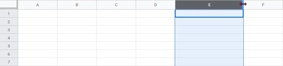
Adjust column width
To adjust the width of a column, follow these steps:
- Hover your cursor at the top right of the column that you want to adjust (over the line that separates that column and the column beside it), where the double arrows that point left and right appear
- Click your mouse and hold the click, then drag your cursor left (to shrink) or right (to expand), and release your click when the column is the desired width.
Adjust row height
To adjust the height of a row, follow these steps:
- Hover your cursor at the left of the row that you want to adjust (over the line that separates that row and the row below it), where the double arrows that point up and down appear
- Click your mouse and hold the click, then drag your cursor upwards (to shrink) or downwards (to expand), and release your click when the row is the desired height.
Note that if there is text in any of the cells within a row, the font size will also determine the row height.
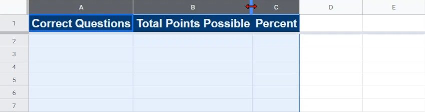
Adjust multiple columns or rows at once
You can also adjust the width of multiple columns or rows at once in Google Sheets.
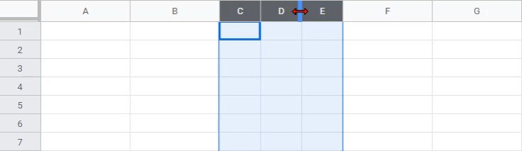
Adjust width of multiple columns
To adjust the width of multiple columns at once, select the columns that you want to adjust, then adjust the width of one of the select columns, and the changes will apply to all of the select columns.
Adjust height of multiple rows
To adjust the height of multiple columns at once, select the rows that you want to adjust, then adjust the height of one of the select rows, and the changes will apply to all of the select rows.
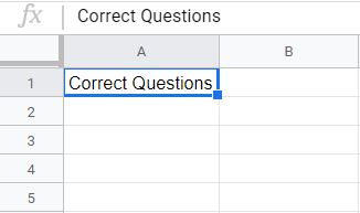
Enter text and numbers into cells (Entering values)
There are multiple ways that you can enter text and numbers into the cells of a spreadsheet.
To enter a value into a cell, select the cell that you want to enter text or numbers into, then do any of the following:
- Start typing, then press enter after typing the desired values
- Or double click on the cell, then start typing (Press enter when done)
- Or click your cursor into the formula bar, then start typing (Press enter when done)
If you choose to simply start typing when a cell is selected, your new text will replace the old text after pressing enter, where the other two methods will allow you to modify existing text.
Cell formatting
Each cell, row, or column can be formatted individually in Google Sheets. Formatting the cells by using color, and different font styles will make your sheet very organized, and professional.
To format a spreadsheet cell, first select the cell or range of cells that you want the formatting changes to apply to, and then apply the formatting that you want.
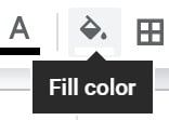
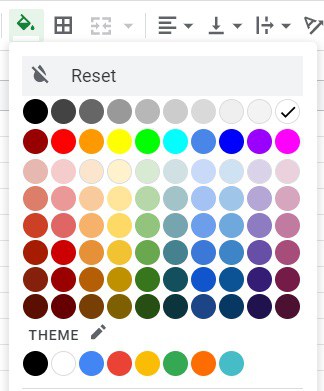
Change the fill color (Background Color)
To change the background color of a cell, select the cell that you want to format, click the “Fill color” menu on the top toolbar (looks like a spilling paint bucket), and then select the color that you want.
Below is an example of the color palette in Google Sheets, which you will see when opening any of the color selection menus.
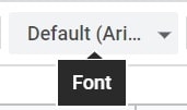
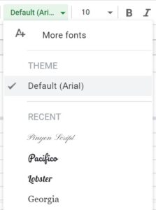
Set the font
To change the font in a cell, select the cell that you want to format, click the “Font” drop-down menu on the top toolbar, and then select the font that you want.
Change the text color
To change the color of the text in Google Sheets, select the cell or cells that you want to modify, click the large letter “A” on the top toolbar to open the “Text color” menu, and then select the color that you want your text to be.
Change the font size
To change the size of the font in Google Sheets, select the cell or cells that you want to modify, click the “Font size” drop-down menu on the top toolbar (directly to the right of the “Font” selection), and then select the size of font that you want to use.
Set the font style
To change the styling of the font in Google Sheets (bold, italic, etc.), select the cell or cells that you want to modify, and then click “bold” or another desired font style on the top toolbar.
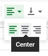
Align the text / values
To change the alignment of the cell contents in Google sheets, select the cell or cells that you want to align, then open the alignment menu on the top toolbar and either select, “Left”, “Center”, or “Right”.
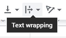
Wrap text in the cells
In a spreadsheet you can “Wrap” text, so that when the text reaches the end of the cell it will continue on a new line.
To wrap the text inside cells, select the cell or cells that you want to wrap, then open the “Text Wrapping” menu on the top toolbar, and then select “Wrap”.
Automatically adjust column width
In your spreadsheet, if you want you can automatically adjust the width of the columns (autofit) so that the columns fit the text inside them. This feature is called “Fit to data”, and although it can be accessed via menus, the easiest way to use it is by using the shortcut described below.
To automatically adjust column width, follow these steps:
- Select the column or columns that you want to adjust
- Hover your cursor at the top right of any of the select columns, over the barrier that separates the column to be adjusted and the column to the right of it, where the the double arrows that point left and right appear
- Double click your mouse, and all of the selected columns will adjust to fit the longest string of text in each column
Copy and paste cells
Copying and pasting cells makes completing spreadsheet tasks much faster and easier. First let’s go over simple copying and pasting, and then later I’ll show you what happens when you copy and paste cells that have formulas in them.
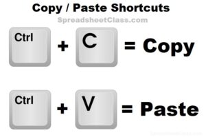
The easiest way to copy and paste, is by using the keyboard shortcuts that are described and displayed, below.
To copy and paste cells, follow these steps:
- Select the cell or range of cells that you want to copy
- Hold the “Ctrl” key on the keyboard, and then press “C”, to copy the cell
- Select the cell where you want to paste your selection
- Hold the “Ctrl” key on the keyboard, and then press “V”, to paste the selection
After copying a cell, you will see a dotted line appear around the cell that has been copied (or the range that was copied).
When you copy and paste a cell that does not have a formula in it, Google Sheets will copy the contents and formatting of the cell, exactly.
If you want to copy and paste only values, without transferring formulas or formatting, hold “Ctrl” on the keyboard and then press “C” to copy the selection like normal, but then hold “Ctrl” AND “Shift” on the keyboard, and then press “V” to paste only values.
The shortcut Ctrl + Shift + V will paste only values in Google Sheets.
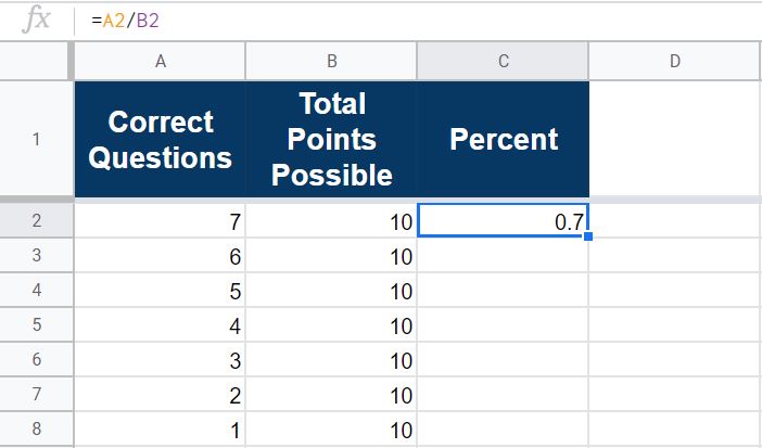
How to enter formulas
Formulas allow you to do a wide array of very useful tasks in a spreadsheet.
To enter a formula in a Google spreadsheet, follow these steps:
- Select the cell that you want to enter a formula into
- Type an equals sign
- Type a formula or function, such as =A2/B2 (Cell A2 divided by cell B2)
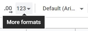
Change the format of the cell values (i.e. Percentage)
Another way that you can change the formatting of the cells in a spreadsheet, is by changing the formatting of the values (contents of the cell such as text or numbers).
To change the formatting of the values in a Google spreadsheet (For example: “Plain text”, “Number”, “Currency, “Percent”), follow these steps:
- Select the cell or range of cells that you want to apply the formatting to
- On the top toolbar, open the “More formats” menu (Button that says “123”)
- Select the format that you want the cell values to be in, such as “Percent”
Copy and paste formulas
We already went over what happens when you copy and paste cells that have normal values entered into them, such as text and numbers, but now let’s go over how to copy and paste formulas in your spreadsheet.
To copy and paste formulas in a Google spreadsheet, follow these steps:
- Select the cell that contains the formula which you want to copy
- Hold “Ctrl” on the keyboard and then press the “C” key, to copy the cell
- Select the cell where you want to copy the formula to
- Hold “Ctrl” on the keyboard and then press the “V” key to paste the selection / formula
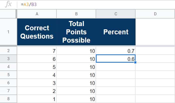
When you copy and paste a formula, the references to cells / cell ranges will adjust when the formula is pasted into a new cell.
When you copy and paste the formula to the right or left, the column references will change.
When you copy and paste a formula up or down, the row references will change.
For example, as shown in the image above, when the division formula was copied from cell C2 and then pasted into cell C3, the formula changed from =A2/B2 to =A3/B3.
In most cases you will want your formula references to change when you copy and paste, but in some cases you will want to stop this from happening, and I will show you how to do this later.
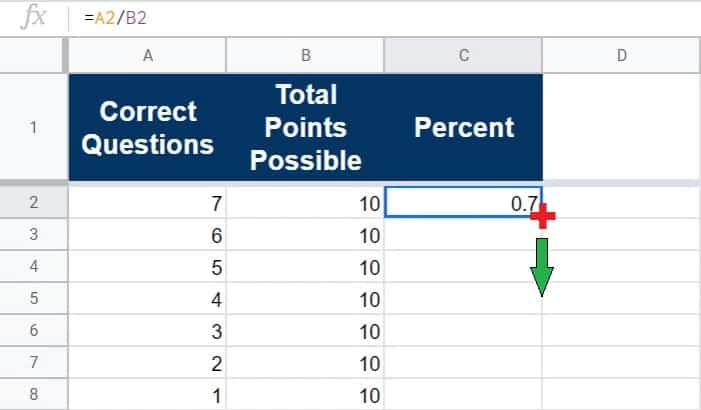
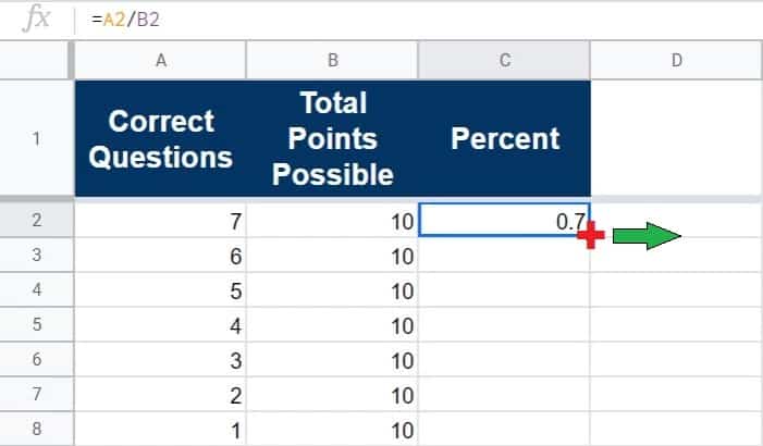
Use autofill / fill down to copy formulas
Copying and pasting is not the only way to copy formulas into other cells. You can also use “Autofill” to quickly copy formulas. Autofill will allow you to fill formulas downwards, or to the right. Let’s go over using “Fill down”.
To use autofill / fill down to copy your formulas downwards, follow these steps:
- Select the cell that contains the formula that you want to copy
- Hover your cursor at the bottom right corner of that cell, until the cross / plus sign (+) appears (this is called the “fill handle”)
- Click your mouse, hold the click, and then drag your cursor downwards
- Release your click when you reach the last cell that you want the formula to be copied into
Just like with copying and pasting your formulas, using autofill will adjust your cell references when the formula is copied into new cells.
Fill formulas to the right
You can also use autofill to copy formulas to the right.
To use autofill / fill right to copy your formulas to the right, follow these steps:
- Select the cell that contains the formula that you want to copy
- Hover your cursor near the bottom right corner of the selected cell, until the cross / plus sign (+) appears (Named the “fill handle”)
- Click your mouse, hold the click, and then drag your cursor to the right
- Release your click when you reach the last cell that you want the formula to be copied into
Delete cell contents
To delete the contents of a spreadsheet cell, select the cell or range of cells that you want to delete the contents of, then press the “Delete” key on the keyboard.
This content was originally created by SpreadsheetClass.com

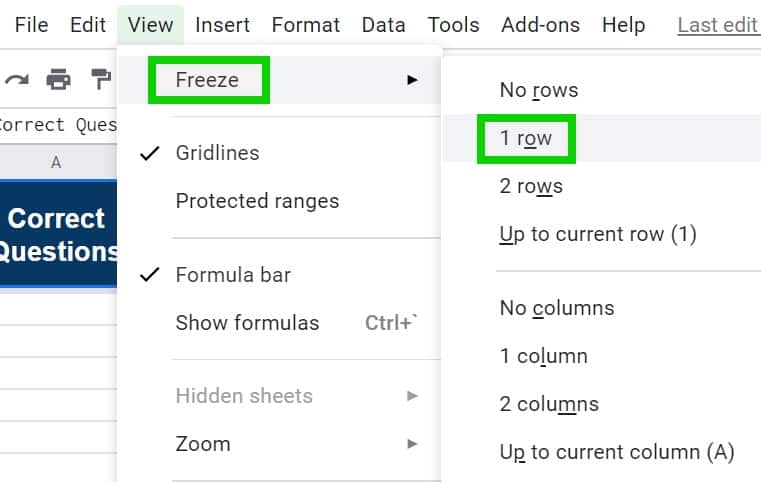
Freeze rows and columns
You can freeze rows and columns in Google Sheets, so that when you scroll, the frozen columns will remain in view at the left side of the spreadsheet, and the frozen rows will remain in view at the top of the spreadsheet.
To freeze rows and / or columns in your spreadsheet, follow these steps:
- On the top toolbar, click “View”
- Hover your cursor over “Freeze”
- Select the number of columns or rows that you want to freeze
Add new rows and columns
You can choose to add rows at the bottom of your Google spreadsheet, or you can also add rows or add columns to a specified location.
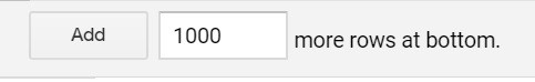
To insert rows at the bottom of the sheet, follow these steps:
- Scroll down to the bottom of the sheet
- Specify the number of rows to add (Default is 1,000)
- Click “Add”
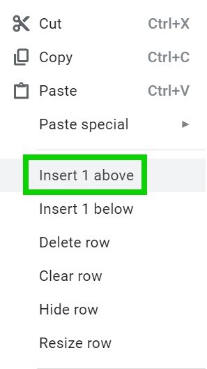
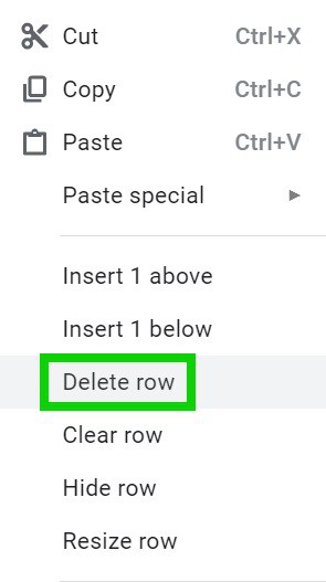
To insert a new row at a specified location, follow these steps:
- Right-click a row that is either directly above or below the location where you want to add a row. (Select multiple rows before right-clicking, if you want to add multiple rows)
- Click “Insert 1 above” or “Insert 1 below”
To insert a new column at a specified location, follow these steps:
- Right-click a column that is either directly to the left or the right of the location where you want to add a column. (Select multiple columns before right-clicking, if you want to add multiple columns)
- Click “Insert 1 left” or “Insert 1 right”
Delete columns and rows
To delete rows in Google Sheets, select the row(s) that you want to delete, right-click on the selected row, then click “Delete row”
To delete columns in Google Sheets, select the column(s) that you want to delete, right-click on the selected column, then click “Delete column”
Absolute and relative cell references (Locking references)
If you want to “lock” your cell references in your formula, so that they do not change when you copy and paste the formula into other cells, there is an easy way to do this in Google Sheets.
To lock the references in your formula, type a dollar sign before the column letter or the row number that you want to remain the same when you copy and paste your formula.
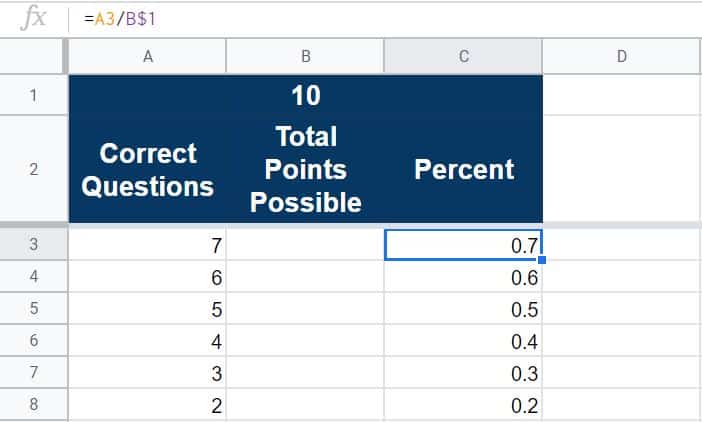
For example, the formula shown above =A3/B$1 has a dollar sign before the row number of the reference to cell B1, which means that as the formula is copied and pasted downwards, the row reference will not change, and the formula will continue referring to cell B1.
As you can see in the example above, the “Total Points Possible” is listed in a single cell (B1), and this cell is referred to by each formula that was copied and pasted downwards, because of where the dollar sign is placed.
Relative references
Relative references WILL change when formulas are copied. These are normal references that do not contain dollar signs, such as =A1.
Absolute references
Absolute references do NOT change when formulas are copied. These references contain a dollar sign before the specified row / column, such as =$A$1.
Mathematical operators (Addition, subtraction, multiplication, division)
In Google Sheets, there are actual functions for performing mathematics in your spreadsheet (i.e. = ADD or SUBTRACT), but these functions are not used very often, due to the existence of mathematical operators.
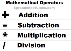
To do math in a Google spreadsheet, use the following mathematical operators:
- Addition: To add, use a plus sign (+). For example: =1+2 or =A1+B1
- Subtraction: To subtract, use a minus sign (-). For example: =2-1 or =B1-A1
- Multiplication: To multiply, use an asterisk (*). For example: =5*7 or =C1*D3
- Division: To divide, use a forward slash (/). For example: =35/7 or =K2/D3
Keyboard shortcuts
There are several keyboard shortcuts in Google Sheets that will make your spreadsheet work much faster and easier. Some of the most useful shortcuts are those that help you select cells quickly, and those that help you fill formulas quickly.
Select cells to bottom of column shortcut
To select all of the cells to the bottom of a column (or to the bottom of the data if the cells are not blank), starting at a specified cell, follow these steps:
- Select the cell that is at the top of the range that you want to select
- Hold “Ctrl” on the keyboard
- Press the down arrow key
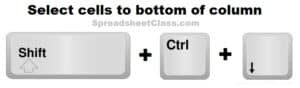
This will select all of the cells below the current cell… to the bottom of the column if the cells are blank, or to the bottom of the data / non-empty cells if there is data in the cells.
Autofill shortcuts
In addition to being able to use the fill handle / autofill to fill formulas downwards and to the right, Google Sheets provides shortcuts for these features as well.
Use the selection shortcut described above to help you select ranges quickly before using the autofill shortcuts.
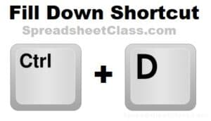
Fill down shortcut
To use the keyboard shortcut to fill formulas down in your Google spreadsheet, follow these steps:
- Select the range that you want to fill formulas with, where the top cell in the selected range contains the formula that you want to copy downwards
- Hold “Ctrl” on the keyboard
- Press the “D” key
This will quickly fill / copy the formula in the top cell of the selected range, down to the bottom of the selected range, without having to take the time to drag the fill handle.
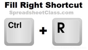
Fill right shortcut
To use the keyboard shortcut to fill formulas right in your Google spreadsheet, follow these steps:
- Select the range that you want to fill formulas with, where the cell that is farthest to the left in the selected range, contains the formula that you want to copy to the right
- Hold “Ctrl” on the keyboard
- Press the “R” key
Extend formulas by using a single formula
There is another easy way to apply your formulas to an entire range, column, or row in Google Sheets, by using ARRAYFORMULA to extend the functionality of a formula throughout multiple cells, by using a single formula in a single cell.
For the example below, we will use a division formula.
To extend a formula through a range by using a single formula, follow these steps:
- Select the cell that contains the formula that you want to extend downwards or to the right
- Type =ARRAYFORMULA( to begin the ARRAYFORMULA function
- Type a formula like you normally would, but then change the cell references to column references, for example this division formula =ARRAYFORMULA(A3:A/B$1)
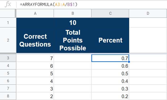
This formula will apply the division formula to the entire column, starting at row 3.
Notice that the reference to cell B1 (B$1) was kept as a single cell reference with a dollar sign listed before the row, which allows the formula to continue referring to cell B1 as the formula is extended downwards.
Cell references (Referring to a single cell)
The simplest formula is a cell reference, which refers to the value that is in a single cell, and displays it in another cell.
To refer to a cell in your spreadsheet with a formula, follow these steps:
- Select the cell that you want to enter your formula / cell reference into, such as cell D2
- Type an equals sign (=)
- Type the address of the cell that you want to refer to, such as B2. The full formula will now look like this: =B2
- Press “Enter” on the keyboard
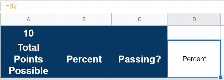
If entered into cell D2, the formula above will display the value that is in cell B2, inside of cell D2.
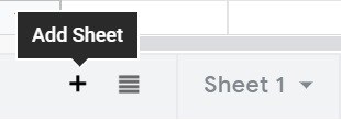
Add new tabs
To add new tabs to your Google spreadsheet, click the plus sign on the bottom left, to the left of the tabs names.
Refer to cells from another sheet
You can also refer to cells from other tabs if you want.
To refer to a a cell from another tab, follow these steps:
- Select the cell that you want to enter your formula / cell reference into
- Type an equals sign (=)
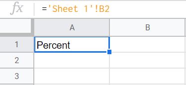
- Type the name of the tab that contains the cell that you want to reference. If the tab name contains a space, you must put the tab name inside of apostrophes, like this =’Sheet 1′
- Type an exclamation point (!)
- Type the address of the cell that you want to refer to, such as B2.The full formula will now look like this: =’Sheet 1′!B2
- Press “Enter” on the keyboard
Again, note that you must include an apostrophe before and after the tab name, if the tab name contains a space in it.
You may include the apostrophes with tab names that do not contain a space and the formula will still function properly.
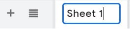
Rename tabs
To rename a tab in Google Sheets, right-click on the tab that you want to rename, and then click “Rename” (Or simply double-click on the tab name), type the new tab name, then press “Enter” on the keyboard.
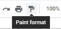
Copy formatting with “Paint Format”
If you only want to copy the formatting of one cell / range to another, without copying the values or the formulas, you can do this with the “Paint format” feature.
To copy formatting from one cell or range to another cell or range, follow these steps:
- Select the cell or range of cells that contain the formatting that you want to copy
- On the top toolbar, click the “Paint format” button, which looks like a paint roller
- Select the cell that you want to transfer the formatting to, and if you had selected a range of cells before clicking “Paint format”, then click the cell that is at the top left of the range that you want to transfer the formatting to
Refer to an entire column with a single formula
In addition to being able to refer to cells, you can also refer to range, rows, and columns in Google Sheets, by using the ARRAYFORMULA function.
To refer to a range of cells with a single formula, follow these steps:
- Select the cell where you want to enter your formula / begin your reference, such as cell D2
- Type =ARRAYFORMULA(
- Type the range that you want to refer to, such as B2:B. The full formula should now look like this =ARRAYFORMULA(B2:B)
- Press “Enter” on the keyboard
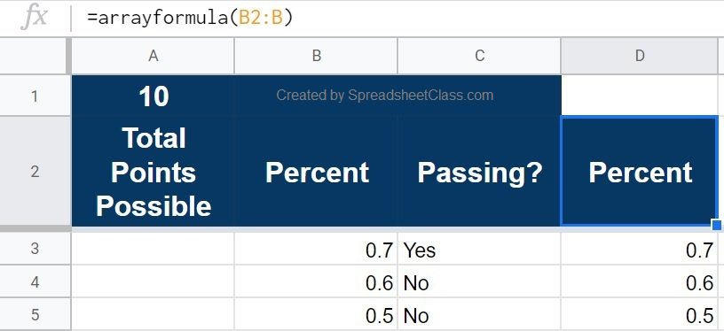
If entered into cell D2, the formula above will display the values that are in column B, inside of column D, starting at row 2.
Move cells, rows, and columns
To move a cell, row, or column in Google Sheets, follow these steps:
- Select the cell, row, or column that you want to move
- Hover your cursor near the top of the cell or column that you want to move, or at the right of the row that you want to move, and your cursor will turn into hand, when your cursor is in the correct position
- Click your mouse, hold your click, and drag your cursor to the location that you want to move the selection to
- Release your click when your cursor is hovering over the place that you want to move the selection to

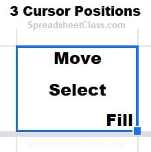
The 3 cursor positions (Select, move, and fill)
As a quick review, let’s go over the 3 different positions that your cursor can be in before clicking within a cell, and what these 3 different positions are for.
- Select: Click in the middle of the cell, where the pointer displays, to select the cell
- Move: Click near the top of the cell, where the hand appears, to move the cell
- Fill: Click at the bottom right corner of the cell, where the cross / plus sign appears, to use autofill
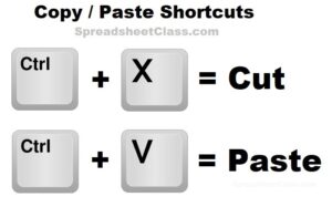
Cut cells, rows, and columns
Cutting and pasting cells, rows, and columns has the same effect that moving them does.
To cut and paste a cell, row, or column, follow these steps:
- Select the cell, row, or column that you want to cut and then paste into another location
- Hold “Ctrl” on the keyboard, and then press “X” to cut the selection
- Select the cell, row, or column where you want to paste the selection
- Hold “Ctrl” on the keyboard, and then press “V” to paste the selection
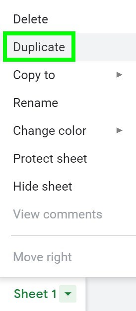
Duplicate tabs
To duplicate a tab in Google Sheets, right-click on the tab that you want to duplicate, and then click “Duplicate”
Delete tabs
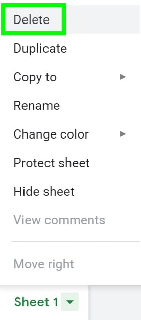
To delete a tab in Google Sheets, right-click on the tab that you want to delete, and the click “Delete”
Use the IF function (If / Then statement)
The IF function is a very common and very useful function in Google Sheets. With the IF function, you set a condition, and then you specify what value or formula to use if the condition is met (TRUE), and what value or formula to use if the condition is not met (FALSE).
In the example below, we will use the IF function to check whether or not a student’s grade is passing, where the formula will display the word “Yes” if the score is at or above 60% (0.6), and where the word “No” will display if the score is below 60%.
To use the IF function to create and IF / THEN statement in Google Sheets, follow these steps:
- Select the cell that you want to enter your formula into
- Type =IF(
- Type a “condition” that compares two values / cells, such as B3>=0.6 (i.e. if cell B3 is greater than or equal to 0.6)
- Type a comma, and then enter the value (or cell reference) that you want to display if the condition is TRUE, such as “Yes”
- Type a comma, and then enter the value (or cell reference) that you want to display if the condition is FALSE, such as “No”. The full formula should now look like this: =IF(B3>=0.6, “Yes”, “No”)
- Press “Enter” on the keyboard
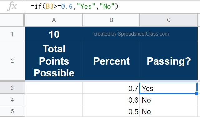
The formula above will display the word “Yes” if the score in cell B3 is greater than or equal to 0.6, and will display the word “No” if the score in cell B3 is less than 0.6.