Math in Google Sheets: Add, Sum, Subtract, Multiply, Divide, Square

One of the most useful things that you can do with Google Sheets, is mathematics. Whether you are simply wanting to solve simple math problems, or whether you have calculations that need to be performed on a set of data, doing math in a Google spreadsheet is very easy if you know the right symbols to use.

To do math in a Google spreadsheet, follow these steps:

1. Type an equals sign in a cell (=)
2. Type a number, or a cell reference (of a cell that contains a number)
3. Then use one of the following mathematical operators  + (Plus),  – (Minus),  * (Multiply),  / (Divide)
4. Type another number or cell reference
5. Press "Enter" on the keyboard

Scroll down to check out the detailed examples and see a wide variety of ways that you can do math in a Google spreadsheet.

In this article I am going to show you how to do math in a Google Spreadsheet, by using ordinary numbers and cell references… and I will also show you the difference between mathematical functions, and mathematical operators.

Click here to get your Google Sheets cheat sheet

Or click here to take the dashboards course

Spreadsheet math: Functions Vs. Operators

If you are new to using Google Sheets formulas, it can be very tempting to use the mathematical functions such as =Add, =Subtract, =Minus, =Divide… and these functions do work… but it is much easier and more common to use spreadsheet operators when doing Addition, Subtraction, Multiplication, and Division in Google Sheets (and squaring too).

Some of these mathematical operators (listed below) are very intuitive, such as Plus (+) and Minus (-), however not all all super obvious, such as the symbol/operator multiplication, which you may think would be the letter "x"… but is actually an asterisk (*).

For summing and square rooting, functions are required for doing this type of math problem instead of operators.

Mathematical spreadsheet operators

• Plus sign (+)  ~  Addition
• Minus sign (-)  ~  Subtraction
• Asterisk (*)  ~  Multiplication
• Forward Slash (/)  ~  Division
• Caret (^)  ~  Exponent

Mathematical spreadsheet functions

• =ADD(  ~  Addition
• =MINUS(  ~  Subtraction
• =MULTIPLY(  ~  Multiplication
• =DIVIDE(  ~  Division
• =SUM(  ~  Summing
• =POWER(  ~  Exponent / Power
• =SQRT(  ~  Square Root

Check out this math problem solver template to easily solve a variety of basic – advanced math problems.

Or check out the math problem generator to quickly create math problems, or to take math test right in a spreadsheet!

Order of operations in a spreadsheet

The order of operations that is taught in normal math classes, also apply in a Google Spreadsheet. The easiest way to make sure that your mathematical formulas are solved in the order that you expect, is to use more parentheses to isolate your needed numbers/terms

The order of operations in a spreadsheet goes as follows:

1. P (Parentheses)
2. E (Exponents)
3. M (Multiplication)
4. D (Division)
5. A (Addition)
6. S (Subtraction)

Here is an example of how the order of operations applies to a math problem:

1. =(6-3)+2^2/4*4-1
2. =(3)+2^2/4*4-1
3. =(3)+4/4*4-1
4. =(3)+1*4-1
5. =(3)+4-1
6. =7-1
7. =6

Using plain numbers vs. cell references

While setting up math formulas in your Google spreadsheet, you can type numbers directly into the formula, or you can also refer to a cell that has a number inside of it…. or you can use a mix of the two where needed.

The big advantage to using cell references in your formulas, is that you can easily change the number inside of the cell, and therefore the number in your formula… without having to alter the formula itself. This is made even more useful when you have multiple formulas that use the same cell reference.

Whether you should type the numbers directly into the formula, or if you should enter the numbers into cells and then refer to those cells in your formula… all depends on your specific task. If you plan to change a number quite frequently, then it is best to use a cell reference. But if you are applying a constant in your formula that will not change, it may be better just to type the number in the formula.

There are several examples of this shown below with images included, but here is a quick explanation of using cell references vs. plain numbers in mathematical spreadsheet formulas.

Doing spreadsheet math by using only numbers

For example, if you wanted to do a simple math problem, using Google Sheets like a calculator, you could type something like the following into a cell:

=27/3

This will display an answer of "9", in the cell.

Spreadsheet math using cell references

But if you want you can also enter the numbers into cells, and do math by referring to those cells. A cell reference is a letter followed by a number… the letter refers to the column, and the number refers to the row. So for example if you wanted to "refer" to a cell in your formula, you would type the reference or cell address, which again is the column letter followed by the row number. So the very first cell in a spreadsheet, in column A and row 1, as cell A1.

If you entered the number "27" into cell A1, and the number "3" into cell B1, you could use the following formula in any other cell:

=A1/B1

This will also display an answer of "9" in the cell.

Using a mix of numbers and cell references to do math

In many cases you will want to use cell references and numbers, like this.

=A1/3

This will also give an answer of "9", assuming that the number "27" is entered into cell A1.

Applying formulas to multiple cells quickly

You will probably want to be able to apply calculations in your spreadsheet to multiple cells easily and quickly, and so I want to show you two ways of doing this. (The final examples in this lesson will demonstrate both of these methods with an image included).

Option 1: After entering a math formula in a cell, copy and paste the cell/formula into the cell(s) below, and the formula will be copied into each individual cell. If there are cell references in your formula, they will adjust automatically as they are copied into the rows below.

Click here to learn how to quickly copy formulas down an entire column.

Option 2: You can also use the ARRAYFORMULA function to make your mathematical formulas apply to multiple cells. With ARRAYFORMULA, you can apply a single formula to multiple cells or an entire column.

How to add in Google Sheets

Let's begin with the different ways to add in Google Sheets. I'll show you how to add by using ordinary numbers, as well as by using cell references, and then I'll show you how to add more than two cells together.

To add in Google Sheets simply type an equals sign in a cell (=), then type the numbers or cells (reference) that you want to add, separated by a plus sign (+), and then press "Enter".

Here are three examples of addition formulas:

1. =25+25
2. =A1+25
3. =A1+B1

Adding numbers

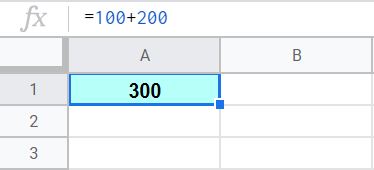
The formula below does not have any cell references, and simply uses plain numbers to do math in Google Sheets, kind of like using a calculator.

Pick any cell in your sheet, type the formula below, and then press "Enter".

=100+200

The cell should display an answer of "300", as shown below.

Adding cells with numbers

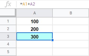
Now let's add by using cell references. Instead of typing numbers directly into our formula, this time we are referring to cells that have numbers inside of them, and telling the formula to add the numbers that are in those cells.

Follow these steps to add in Google Sheets:

1. Click on cell A1, then type the number "100", and then press "Enter"
2. Click on cell A2, then type the number "200", and then press "Enter"
3. Click on cell A3, then type "=A1+A2", and then press "Enter"
4. Cell A3 should now display an answer of "300"

Formula shown below: =A1+A2

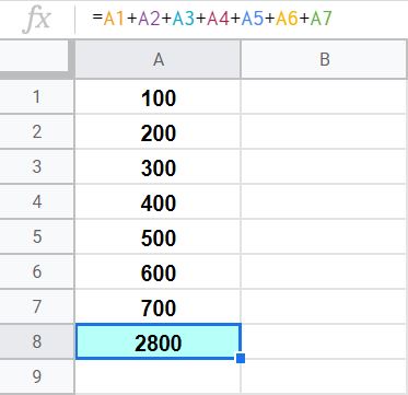
Adding multiple cells

You can also add more than two cells together in your spreadsheet. Simply continue typing the cell references that you want to add, separated by plus signs, and then press "Enter" when your formula is complete.

After typing a plus sign, or any other mathematical operator for that matter, you can also click on the cell that you want to refer to rather than having to type the reference.

Formula shown below: =A1+A2+A3+A4+A5+A6+A7

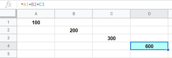
Adding multiple non-adjacent cells

If the cells that you are adding together are all in the same column or row, the easiest way to add them is by "summing" them, which I will show you in just a moment… but when the cells that you are adding are not adjacent, this is when adding multiple, individual cells becomes extremely useful.

If your sheet has numbers entered in varying locations that you want to add together, you can do so by using a formula like one that is shown in the example below.

Formula used in example: =A1+B2+C3

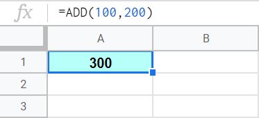
Using the ADD function to add

Using the ADD function to add is much less common and less useful than using the plus sign operator, but here is an example that shows how to use it in case you have a need for it.

Formula shown below: =ADD(100,200)

How to sum in Google Sheets

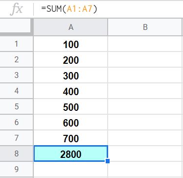
The SUM function is an extremely useful formula that will allow you to sum entire rows, columns, or specified ranges.

To sum in Google Sheets, begin by typing "=Sum(", then type the range of cells that you want to sum, for example "B1:B100", type a closing parentheses ")", and then press "Enter".

Let's say that you have a column of numbers that you want to add, but you don't want to have to have a long formula that adds lots of individual cells. This is where you would use the SUM function.

To total an entire column in a Google spreadsheet, do either of the following:

1. Use the cell at the top of the column to enter a formula like this, which sums all of the cells below it: =SUM(C1:C)
2. Or use a cell that is below the range that you want to sum, and enter a formula that contains the range of cells that are above it. In other words, for example if your SUM formula is in cell C100, then to sum the numbers in column A that are above your formula, make sure you specify an ending row in the range that is less than 100, like this: =SUM(C1:C99)

Formula shown in example image below: =SUM(A1:A7)

Note: If the range in your sum formula contains the cell that your formula is entered in, it will cause a circular dependency error.

How to subtract in Google Sheets

Now let's go over the different ways to subtract in a Google spreadsheet. Again I will show you how to subtract by using numbers alone, and I will also show you how to subtract with cell references.

To subtract in Google Sheets, type an equals sign in a cell (=), then type the numbers or cell references (i.e. A1) that you want to subtract with a minus sign (-) between them, and then press "Enter".

Here are three examples of subtraction formulas:

1. =100-50
2. =A1-50
3. =A1-B1

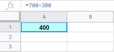
Subtract numbers

Here is an example that shows how to subtract by simply using numbers directly in the formula.

Formula shown in example below: =700-300

After entering the formula above into a cell in your spreadsheet, and the cell will display an answer of "400".

Subtract cells with numbers

You can also use cell references to subtract… where the numbers that you want to subtract from one another are entered in cells, and where you then refer to those cells within the formula to perform your calculation. Using cell references to subtract will allow you to change the numbers that your formula refers to very quickly and easily, without having to modify your formula.

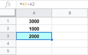
Follow these steps to subtract in Google Sheets:

1. Click on cell A1, then type the number "3000", and then press "Enter"
2. Click on cell A2, then type the number "1000", and then press "enter"
3. Click on cell A3, then type "=A1-A2", and then press "Enter"
4. Cell A3 should now display an answer of "2000"

Example formula: =A1-A2

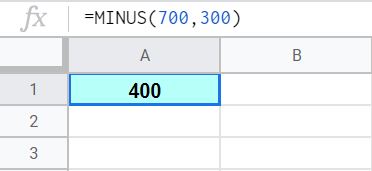
Using the MINUS function to subtract

Here is an example that shows how to subtract by using the MINUS function.

Formula shown below: =MINUS(700,300)

How to multiply in Google Sheets

Now let's go over how to multiply in a Google spreadsheet. Just like with addition and subtraction, you can choose whether you want to use ordinary numbers in your formula, or whether you want to use cell references… or a mix of the two.

To multiply in a Google spreadsheet, first type an equals sign in a cell (=) , then type the numbers or cell references that you want to multiply with an asterisk (*) separating them, and then press "Enter".

Here are three quick examples of multiplication formulas:

1. =10*10
2. =A1*10
3. =A1*A2

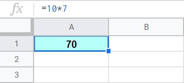
Multiply numbers

If you want, to multiply you can use your spreadsheet like a calculator, and simply type a formula like the one shown below, which does not use any cell references and had its numbers typed directly into the formula bar.

Formula shown in example: =10*7

Enter the formula above into a cell in your sheet, and the cell will display an answer of "70".

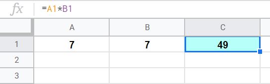
Multiply cells with numbers

Again just like with addition and subtraction, you can use cell references in your multiplication formulas, where the numbers that you want to multiply are entered into individual cells, and where your formula refers to those cells to designate the values to be multiplied.

Follow these steps to multiply in Google Sheets:

1. Click on cell A1, then type the number "7", and then press "Enter"
2. Click on cell B1, then type the number "7", and then press "Enter"
3. Click on cell C1, then type "=A1*B1", and then press "Enter"
4. Cell C1 should now display an answer of "49"

Formula shown below: =A1*B1

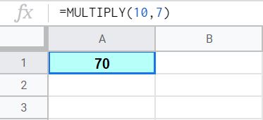
Using the MULTIPLY function to multiply

The example below shows how to multiply by using the MULTIPLY function. However it is much more common and easy to use the operator method shown above.

Formula shown below: =MULTIPLY(10,7)

How to divide in Google Sheets

Now I'll show you how to divide in your Google spreadsheet. Once again, I'll show you the difference between using ordinary numbers vs. using cell references to divide… and I'll also show you the difference between using an operator vs. a function to divide.

To divide in a Google spreadsheet, start by tying an equals sign in a cell (=), then type the numbers (or references to cells with numbers) that you want to divide, separate them with a forward slash (/), and then press "Enter".

Here are three simple examples of division formulas:

1. =75/3
2. =A1/3
3. =A1/A2

Note that just like when using a calculator, you cannot successfully divide by 0 in a spreadsheet. If your denominator (number "on bottom" or after the slash) is 0, your division formula will display a #DIV/0 error. This error can be handled by using the IFERROR function which will allow you to specify what value should be displayed if the formula has an error.

Here are two examples of handling the #DIV/0 error:

1. =IFERROR(C1/C2,0)
2. =IFERROR(C1/C2,"Error")

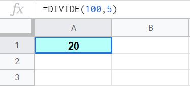
Divide numbers

Here is an example that shows how to divide by using numbers only, without referring to any cells in the sheet.

Formula shown below: =100/5

Enter the formula above into any cell in your sheet, and the cell should display an answer of "20".

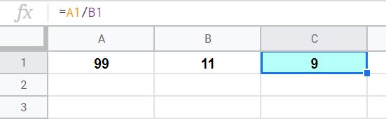
Divide cells with numbers

If you want, you can enter the numbers that you want to divide into individual spreadsheet cells, and then refer to those cells in your division formula. This will be especially useful if you plan to change one or more of the values in your formula over time.

Follow these steps to divide in Google Sheets:

1. Click on cell A1, then type the number "99", and then press "Enter"
2. Click on cell B1, then type the number "11", and then press "Enter"
3. Click on cell C1, then type "=A1/B1", and then press "Enter"
4. Cell C1 should now display an answer of "9"

Formula shown below: =A1/B1

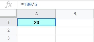
Using the DIVIDE function to divide

This example will show you how to divide in a Google spreadsheet by using the DIVIDE function.

Formula shown below: =DIVIDE(100,5)

This content was originally created and written by SpreadsheetClass.com

How to square numbers in Google Sheets

Squaring numbers in a Google spreadsheet is just as easy as the four basic mathematical operations that we have went over so far.

In a spreadsheet, a caret "^", symbolizes "To the power of", meaning that this is how we express an exponent in a spreadsheet… by combining a caret with a number. So "^2" means "To the second power", or simply "squared".

You can also choose any other number than 2 to raise a number to a specified power/exponent, such as cubing: "^3"

To square numbers in Google Sheets, type a numbers or a cell reference (to a cell containing a number), then type a caret "^", then type the number "2", and then press "Enter".

Here are a couple examples of squaring formulas:

1. =10^2
2. =C1^2

Square numbers

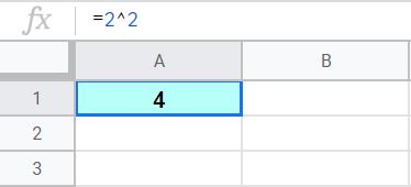
The simplest way to square a number i your spreadsheet, is to simply type a formula like the one below.

Formula shown in the example image below: =2^2

Enter the formula above into any cell in your spreadsheet, and the cell should show an answer of "4".

Square cells with numbers

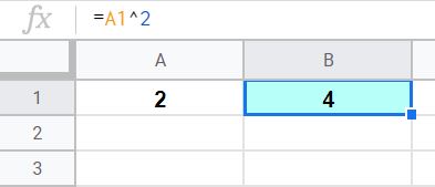
Just like with the other math operations, you can type the number that you want to square into a cell, and the (in another cell) refer to the cell with the number inside it with/in your square formula, as shown below.

Follow these steps to square numbers in Google Sheets:

1. Click on cell A1, then type the number "2", and then press "Enter"
2. Click on cell B1, then type =A1^2, and press "Enter"
3. Cell B1 should now display an answer of "4"

Formula used in the example below: =A1^2

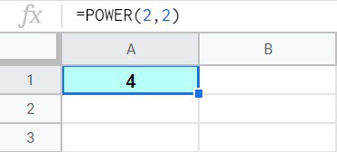
Square using the POWER function

There is also a function that can be used to square, and it is called POWER. This function can also be written as simply POW. Here is an example of how to use this function.

Formula shown below: =POWER(2,2)

Formula alternative: =POW(2,2)

How to square root numbers in Google Sheets

If you need to square root a number in your Google spreadsheet, you can use the SQRT function.

To square root in Google Sheets, in any cell simply type "=SQRT(", then type a number of your choice, type a closing parentheses ")", and then press "Enter".

Here are two examples of square root formulas:

1. =SQRT(9)
2. =SQRT(100)

Square root numbers

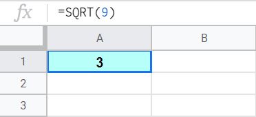
The most simple way to square root a number in your sheet, is to simply enter an ordinary number directly into the SQRT formula, as shown below.

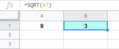
Formula used in example below: =SQRT(9)

Enter the formula shown above into a cell in your spreadsheet, and then the cell should display an answer of "3".

Square root cells with numbers

If you want to use a cell reference to designate the value that you want to square root, so that when you change the number in the cell it also changes your answer… you can do this with the SQRT function as well by simply typing a cell address/reference in the function.

Follow these steps to square root in Google Sheets:

1. Click on cell A1, then type the number "9", and then press "Enter"
2. Click on cell B1, then type =SQRT(A1), and press "Enter"
3. Cell B1 should now display an answer of "3"

Formula used in example below: =SQRT(A1)

How to calculate equations in Google Sheets

Google Sheets can do much more than just simple math problems with two values. You can also set up math equations so that your sheet will automatically solve the equation as you enter/change the variables.

Shown below is how to calculate the circumference and area in your spreadsheet, given a specified radius.

Notice that these equations use numbers and cell references in the formula. The numbers entered directly into the formula, such as 3.14 (pi), which is a constant… and the cell references represent the radius, which is a variable and we want to be able to easily modify.

Circle circumference spreadsheet equation (where A2 is the radius)

=2*3.14*A2

Circle area spreadsheet equation (where A2 is the radius)

=3.14*A2*A2

Alternative formula: =3.14*A2^2

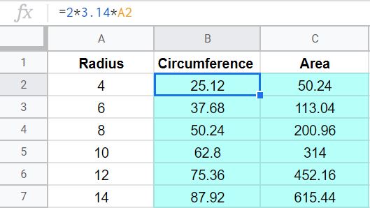
In the image above you can see that the circumference formulas are entered in column B, and that the area formulas are entered in column C.

There is a formula in each blue cell in the image… and each formula refers to the radius that is listed adjacent to it. This was done by copying and pasting the formulas at the top (row 2), into the cells below.

When copying and pasting formulas like this, the cell reference will automatically adjust as the formula is pasted into the next row. This is how the circumference and area formulas each refer to the radius listed in its same row, because every time the formulas are pasted into the next cell below, the cell reference will also adjust by one row.

Below you can see what the formulas will look like as they are copied into the rows below row 2 in the example above.

Copying the circumference formula down the column:

Row 3:   =2*3.14*A3

Row 4:   =2*3.14*A4

Row 5:   =2*3.14*A5

Copying the area formula down the column:

Row 3:   =3.14*A3^2

Row 4:   =3.14*A4^2

Row 5:   =3.14*A5^2

Applying the equations to the entire column:

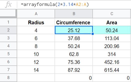
=arrayformula(2*3.14*A2:A)

=arrayformula(3.14*A2:A^2)

How to create equations with multiple operators

Now let's take a look at using an equation that uses multiple types of operators in one formula.

Below is an example that shows a calculation and comparison of two different services and how much each costs depending on the number of hours of service.

Let's say that you are going to hire a photographer. They have a different base cost and a different hourly rate, and you want to know which one will cost the least… again depending on how many hours you will need to hire them for.

To calculate the total cost of service for a given hourly rate, base cost, and number of hours… we will do the following:

Take the hourly rate (Column C) multiplied by the number of hours (Column D), and then add the base cost (Column B).

As you can see in the example image, the first formula is entered into cell E2:

=B2+(C2*D2)

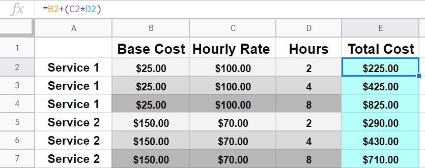
This formula is then copied and pasted into the cells below to make the same calculation for each individual row of data.

Due to the differences in base cost and hourly rate, one service will cost less overall when hired for a short amount of time, and the other service will cost less when hired for a longer period of time.

In this example we can see that photographer 1 is cheaper when hired for 2 hours, but photographer 2 is cheaper when hired for 8 hours. Both photographers are comparable when hired for 4 hours.

Lesson review

Let's summarize the main formulas that we went over in this lesson.

Here are the mathematical formulas in Google Sheets:

Addition formulas in Google Sheets

Add by using cell references

• =A1+A2

Add numbers, without cell references

• =100+200

Add by using the ADD function

• =ADD(100,200)

Sum formula in Google Sheets

• =SUM(A1:A7)

Subtraction formulas in Google Sheets

Subtract by using cell references

• =A1-A2

Subtract numbers, without cell references

• =700-300

Subtract by using the MINUS function

• =MINUS(700,300)

Multiplication formulas in Google Sheets

Multiply by using cell references

• =A1*B1

Multiply numbers, without cell references

• =10*7

Multiply by using the MULTIPLY function

• =MULTIPLY(10,7)

Division formulas in Google Sheets

Divide by using cell references

• =A1/B1

Divide numbers, without cell references

• =100/5

Divide by using the DIVIDE function

• =DIVIDE(100,5)

Square formulas in Google Sheets

Square by using cell references

• =A1^2

Square numbers, without cell references

• =2^2

Square numbers using the POWER function

• =POWER(2,2)
• =POW(2,2)

Square root formulas in Google Sheets

Square root by using cell references

• =SQRT(A1)

Square root numbers, without cell references

• =SQRT(9)

Pop Quiz: Test your knowledge

Answer the questions below about math in Google Sheets, to refine your knowledge! Scroll to the very bottom to find the answers to the quiz.

Question #1

Which of the following formulas adds the numbers "5" and "10" together?

1. =ADD(5,10)
2. =5+10
3. Both

Question #2

Which of the following formulas multiplies the numbers "10" and "30" by each other?

1. =10×30
2. =10*30

Question #3

True or False: The order of operations in traditional math is the same as the order of operations in a spreadsheet (PEMDAS)?

1. True
2. False

Question #4

If the number "4" is entered in cell A1, and the number "3" is entered in cell A2, what is the answer to this formula: =A1-A2?

1. =-1
2. =1

Question #5

Which of the following formulas can be used to add cells A1 through A5?

1. =A1+A2+A3+A4+A5
2. =SUM(A1:A5)
3. Both

Answers to the questions above:

Question 1:  3

Question 2:  2

Question 3:  1

Question 4:  2

Question 5:  3