How to divide in Google Sheets (Divide numbers, cells, columns, & rows)

Google spreadsheets make it very easy to do math, such as dividing numbers, cells, and entire columns / rows. Spreadsheets make dividing easy in so many ways, from being able to do multiple division formulas at once, to being able to use cell references so that your division formula criteria is easily controlled by entering values into cells.

In other words, you can set up your formula once and then it automatically performs the division calculation as the data changes.

In this lesson I will show you how to do all of that and more.

To divide in Google Sheets, follow these steps:

1. Select the cell where you want to create a division formula, then type an equals sign (=)
2. Type the number or the cell reference that contains the number that you want to divide into (numerator)
3. Type a forward slash (/)
4. Type the number or the cell reference that contains the number that you want to divide by (denominator). The final formula will look like this: =100/50 (Or like this for cell references: =A1/A2)
5. Press "Enter" on the keyboard

After following the steps above, Google Sheets will display the result of the division calculation in the cell where you entered the formula.

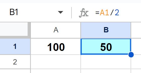
Let's say that you want to divide the value that is in cell A1 (100) by the number "2". To do this simply enter the formula =A1/2 in a cell, then press enter on the keyboard and the formula will display the result. In this case the result would be "50", since 100/2=50 (shown in the image below).

=A1/2

Click here to learn how to do all the different types of math in a Google spreadsheet.

See the detailed examples below that teach a variety of ways to divide in a Google spreadsheet.

Divide symbol / operator

The easiest and most common way to divide in Google Sheets, is by using the divide operator / symbol, which is a forward slash (/).

There is also a DIVIDE function that allows you to divide, but this function is not commonly used, and the operator method is much easier / more versatile, so we will stick to using operators in this lesson.

But here is an example of the DIVIDE function: =DIVIDE(100,A1)

Dividing numbers

First let's go over a basic example of dividing by using numbers that are entered directly into the formula.

Sometimes you may want to do this to simply solve a quick division problem without using cell references. I use numbers entered directly into my division formulas when there is a constant that I want to divide by (i.e. when I know that the numbers in the division formula will stay the same).

To divide numbers in Google Sheets, follow these steps:

1. Select the cell where you want to create a division formula, then type an equals sign (=)
2. Type the number that you want to divide into (numerator)
3. Type a forward slash (/)
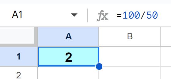
4. Type the number that you want to divide by (denominator). The final formula will look like this: =100/50
5. Press "Enter" on the keyboard

In this case the result would be "2", since 100/50=2 (shown in the image below).

=100/50

Divide by using cell references

Spreadsheets are very useful for doing division, because of the ability to use cell references in your formulas. This allows you to refer to a cell that contains a number, rather than entering numbers directly into the formula.

When you use a cell reference for your division formula, the value inside the cell can easily be changed and the formula will automatically perform the calculation with the new value, making it very fast and easy to do division, especially when you are dividing a large amount of data that changes frequently.

To divide cells in Google Sheets, follow these steps:

1. Select the cell where you want to create a division formula, then type an equals sign (=)
2. Type the cell reference that contains the number that you want to divide into (numerator)
3. Type a forward slash (/)
4. Type the cell reference that contains the number that you want to divide by (denominator). The final formula will look like this: =B1/B2
5. Press "Enter" on the keyboard

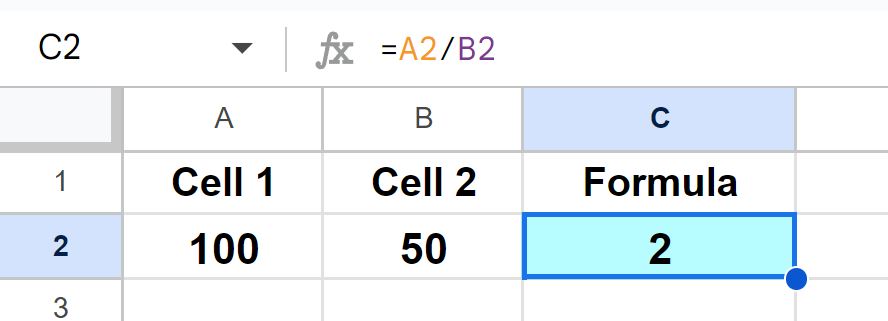
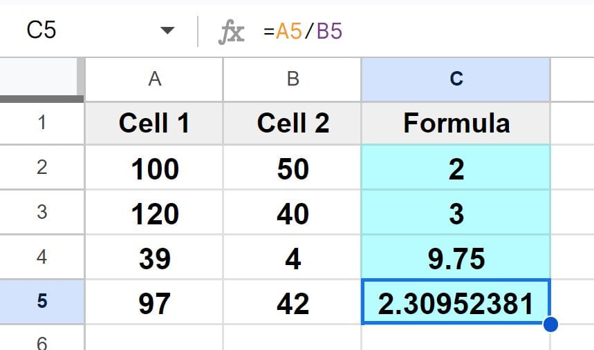
Let's say that you want to divide the value in cell A2 (100) by the value that is in cell B2 (50). To do this simply enter the formula =A2/B2 in a cell, then press enter on the keyboard and the formula will display the result. In this case the result would be "2", since 100/50=2 (shown in the image below).

=A2/B2

Using autofill (or copy / paste) to copy division formulas

If you want to copy your division formula down the column or through a row, this can be done easily by either using autofill or by copying / pasting your formulas.

Later I will show you how to use the ARRAYFORMULA function to apply a division formula to a range of cells by using a single formula, but for now let's go over how to quickly copy individual division formulas.

Method 1: To copy and paste your division formula into other cells, copy the cell with the division formula in it by pressing Ctrl + C on the keyboard, select the cell that you want to copy the formula to, then paste by pressing Ctrl + V on the keyboard.

Method 2: To copy your division formula by using autofill, select the cell that has the formula in it, hover your cursor over the bottom-right corner of the cell until the plus sign appears (the fill handle), click your mouse and hold the click, drag your cursor across the cells that you want to copy the formula into, then release your click when you have selected all of the cells that you want to copy the division formula into.

With both of these methods, Google Sheets will automatically adjust the cell references when the formulas are copied into adjacent cells, so that each new formula is correctly referring to the appropriate column / row.

For example if you enter the formula =A1/2 (in cell B1), and then copy the formula from cell B1 into cell B2, then Google Sheets will automatically adjust the reference so that the new formula will be =A2/2.

So when you copy a formula down the column, the row references will adjust, and when you copy a formula throughout a row, the column references will adjust.

Locking cell references for division formulas

If you have a situation where you want to lock the references in your division formula so that they do not change when you copy them into other cells, use a dollar sign ($) before the reference that you want to lock.

Put a dollar sign before the column letter if you want the column reference to be locked, and put a dollar sign before the row number if you want the row reference to be locked.

• =$A1/2 (Locked column reference)
• =A$1/2 (Locked row reference)
• =$A$1/2 (Locked column + locked row reference)

Below are several detailed examples of using autofill to copy division formulas.

Dividing columns of data with autofill

In this example we will go over how to copy division formulas vertically down a column.

To divide columns in Google Sheets, follow these steps:

1. Enter your division formula in the first cell at the top of the column
2. Select the cell with the formula in it, and hover your cursor over the bottom-right corner of the cell until a plus sign appears
3. Click your mouse and hold the click, then drag your cursor down the column
4. Release your click when you have selected all of the cells that you want to copy your division formula into

As you can see in the image below, the following formula is entered into cell C2:

=A2/B2

We are going to copy the formula down the column into the cells below by using autofill / the fill handle.

First we select cell C2, then hover the cursor over the bottom-right corner of the cell until the plus sign / cross appears, as shown in the image below.

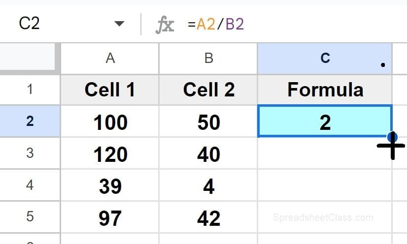
Then click your mouse, hold the click, and drag your cursor downwards until you have reached cell C5, then release your click.

As you can see in the image below, the formula from cell C2 has now been copied into the cells below it, into the range C2:C5. You can also see that the formula in cell C5 has had its row references adjusted, and the formula in cell C5 is A5/B5. This is what we wanted Google Sheets to do, since our references are connected to the correct rows.

Dividing rows of data with autofill

You can also use the fill handle to copy formulas to the left and right in your spreadsheet. Now let's go over how to copy division formulas horizontally through a row.

To divide rows in Google Sheets, follow these steps:

1. Enter your division formula in the first cell on the left of the row
2. Select the cell with the formula in it, and hover your cursor over the bottom-right corner of the cell until a plus sign / cross appears
3. Click your mouse and hold the click, then drag your cursor to the right
4. Release your click when you have selected all of the cells that you want to copy your division formula into

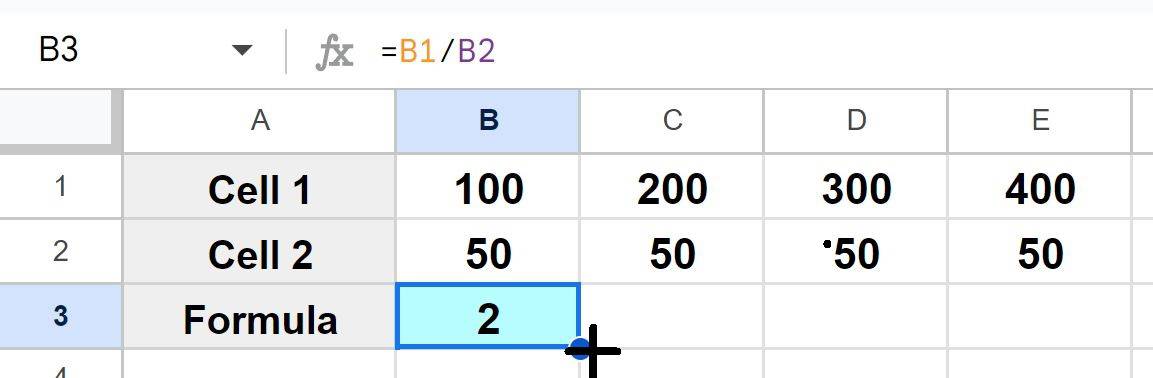
As you can see in the image below, the following formula is entered into cell B3:

=B1/B2

We are going to copy the formula into the cells to the right in the same row, by using autofill / the fill handle.

First we select cell B3, then hover the cursor over the bottom-right corner of the cell until the plus sign / cross appears, as shown in the image below.

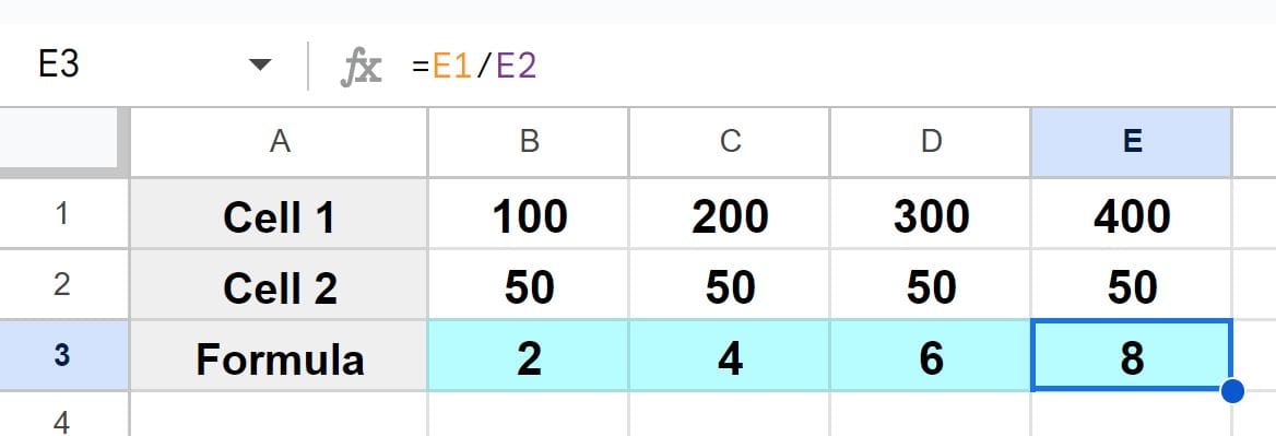
Then click your mouse, hold the click, and drag your cursor to the right until you have reached cell E3, then release your click.

As you can see in the image below, the formula from cell B3 has now been copied into the cells to the right of it, into the range B3:E3. You can also see that the formula in cell E3 has had its column references adjusted, and the formula in cell E3 is E1/E2. This is what we wanted Google Sheets to do, since our references are connected to correct columns.

Using ARRAYFORMULA to extend formulas

There is a very useful formula called ARRAYFORMULA that allows you to perform calculations on an entire range of data, such as dividing entire columns or rows, in a single formula. Here's how to divide entire columns and rows using ARRAYFORMULA.

Dividing entire columns

In this example we will use ARRAYFORMULA to divide an entire column by using a single formula.

To divide entire columns with a single formula, follow these steps:

1. Enter your division formula in a cell at the top of the column, like this: =A2/B2
2. Press Ctrl + Shift + Enter on the keyboard to turn the division formula into an ARRAYFORMULA formula
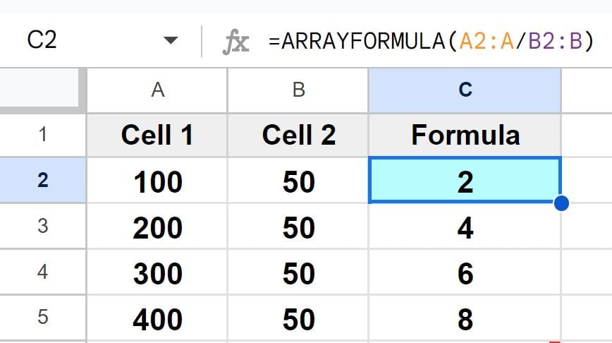
3. Change any cell references to a range / column reference, like this: =ARRAYFORMULA(A2:A/B2:B)
4. Press enter on the keyboard

This formula tells Google Sheets to divide each corresponding cell in column A by the respective cell in column B

As you can see in the image below, the formula in cell C2 is calculating division for the entire range C2:C5 by using a single formula.

Dividing entire rows

In this example we will use ARRAYFORMULA to divide an entire row by using a single formula. This is very similar to dividing entire columns, but in this case we will specify rows for our references rather than columns. Notice how in the previous example the reference looked like this B1:B, but in this example the reference looks like this B1:1.

To divide entire rows with a single formula, follow these steps:

1. Enter your division formula in a cell on the right of the row, like this: =B1/B2
2. Press Ctrl + Shift + Enter on the keyboard to turn the division formula into an ARRAYFORMULA formula
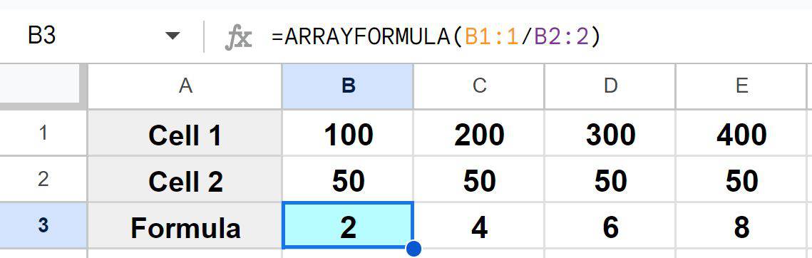
3. Change any cell references to a range / row reference, like this: =ARRAYFORMULA(B1:1/B2:2)
4. Press enter on the keyboard

This formula tells Google Sheets to divide each corresponding cell in row 1 by the respective cell in row 2.

As you can see in the image below, the formula in cell B3 is calculating division for the entire range B3:E3 by using a single formula.

Fixing the divide by zero #DIV/0! error when dividing

When you are dividing in a spreadsheet, occasionally you will encounter the #DIV/0! (divide by zero) error. This error simply means that the formula is trying to divide by zero, or in other words a zero value is in the denominator (bottom part of a division formula).

For example, if you enter the formula =100/A1, where cell A1 is either blank or contains the number 0, this will cause a divide by zero error. If a number is entered into cell A1, the formula will no longer display an error and will display the result of the division formula as desired.

Or you can use the IFERROR function combined with your division formula to remove the error, so that the cell with the formula displays whatever message that you want when an error occurs, like this: =IFERROR(100/A1, "N/A")

The formula above will display the text "N/A" if an error occurs in the division formula.

Sometimes this #DIV/0! error happens when your formula is set up correctly but there is simply no data or the data has zero values… and sometimes this can happen when you incorrectly set up your formula such as referring to the wrong cell or range of cells.

Check carefully to make sure that you are referring to the correct cell(s) with your division formula. If your formula is set up correctly, check to make sure that no data is missing from the cells that you are referring to. There are legitimate cases when the divide by zero error can occur, such as if you are averaging data for each employee but some employees have not had data entered yet.

Now you know all of the different ways to divide in Google Sheets!

Click here to get your Google Sheets cheat sheet

Or click here to take the dashboards course