

Have you ever wanted to divide in your spreadsheet without a remainder, where the answer is a whole number? There are several ways to do this, depending on which function you want to use, and depending on if you want to round up, round down, or round according to normal rounding rules.
The most common way to divide without a remainder is to round down, which essentially means discarding the remainder / decimal value that is attached to a whole number. This allows us to find how many times one number fits into another number “evenly”. But again there may be scenarios where you will want to choose whether you round up or down etc., and in this lesson I will show you how to do exactly that.
To divide without a remainder in Google Sheets, follow these steps:
- Type =ROUNDDOWN( in an empty spreadsheet cell
- Type a number or the cell that contains the number that you want to divide into
- Type a forward slash (/)
- Type the number or the cell that contains the number that you want to divide by
- Press “Enter” on the keyboard. The final formula will look like this: =ROUNDDOWN(10/3) or like this when using cell references: =ROUNDDOWN(A1/A2)
After following the steps, the formula will display the result of the division calculation without a remainder, where only the whole number is displayed and the remainder is discarded.
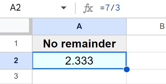
Now let’s go over some examples of the varying ways to divide without a remainder, but first take a look at the image below. As you can see, the formula in cell A2 divides 7 by 3 (=7/3), and this results in an answer of 2.333 (where the decimal keeps going). The remainder is the numbers that come after the decimal, which is what we will be using a variety of formulas to remove when dividing in your Google spreadsheet.
Using the ROUNDDOWN function to divide without a remainder
Let’s go over a basic example of dividing without a remainder, where the numbers are entered directly into the formula. We will use the ROUNDDOWN function to round the result of the calculation down to the nearest whole number, which will effectively “remove” the remainder.
There are two portions to the formula, there is the division calculation (7/3), and the ROUNDDOWN function that is applied. When we put them together the formula looks like this: =ROUNDDOWN(7/3)
7/3 = 2.333
=ROUNDDOWN(7/3) yields and answer of 2.0
This formula will yield an answer of “2”, when the remainder is removed from the result of 7/3.
=ROUNDDOWN(7/3)
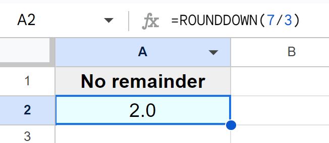
In the image above, you can see that the formula in cell A2 displays the number “2”, after the remainder was removed from the division result.
As you can see in the formula above, the division calculation is put inside the ROUNDDOWN function, which in spreadsheets is called “nesting” a formula. So the division calculation is nested inside the ROUNDDOWN function. Another way of saying this is to say that the ROUNDDOWN function is wrapped around the division calculation.
Note that the formula below does the same thing as the formula above, since the ROUNDDOWN function defaults to zero decimal places if you do not specify the number of decimal places. The formula below specifies zero decimal places, which means that the formula will round down to the nearest whole number, which again is the default if no decimal places are specified at all.
=ROUNDDOWN(7/3,0)
Using cell references when dividing without a remainder
If you want, you can enter the numbers that you are dividing into spreadsheet cells instead of having to enter them directly into the formula. This will make it easy to change the values that the formula calculates.
For example, if you want to divide the number 7 by the number 3, you can enter the number 7 into cell A1, then enter the number 3 into cell A2, and use the formula =A1/A2 to divide the numbers.
In the examples below, we will use this cell reference method as we go over more functions to divide without a remainder.
Using the ROUND function when dividing
In this example, we are going to use the ROUND function to handle the remainder in a different way. The round function follows traditional rounding rules, and so instead of discarding the remainder completely by rounding down, the formula will decide whether to round up or down depending on how close the result of the division calculation is to the next highest or next lowest whole number.
So if the result of the division calculation is 2.1, the ROUND function will round down to the number 2.
If the result of the division calculation is 2.9, the ROUND function will round up to the number 3.
This will allow you to divide without a remainder, where the answer is a whole number, but the whole number that is displayed as a result will depend on whether the function rounds up or down.
As you can see in the image below, there are numbers entered into column A (numbers to divide into / numerator) and column B (numbers to divide by / denominator). So we are going to divide the numbers in column A by the numbers in column B, and then we will use the ROUND function to display a result that is a whole number (where the function rounds to the nearest whole number).
We will use the formula =ROUND(A2/B2) to round the result of the division calculation to the nearest whole number.
=ROUND(A2/B2)
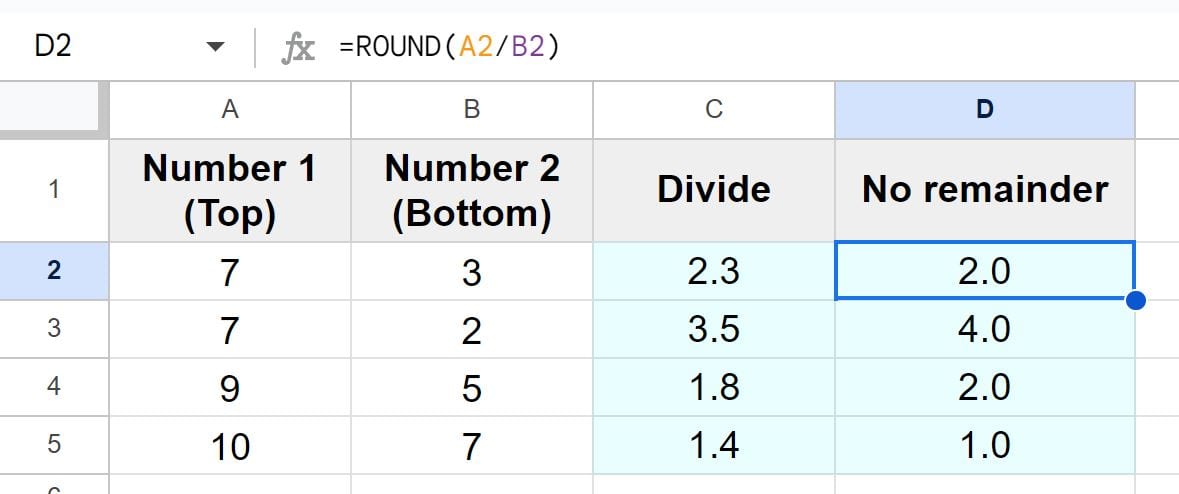
As you can see in the image above, cell D2 displays the number “2”, since the ROUND function rounded down from 2.3
Cell D3 displays the number “4”, since the ROUND function rounded up from 3.5
Cell D4 displays the number “2”, since the ROUND function rounded up from 1.8
Note that the formula below does the same thing as the formula above, since the ROUND function defaults to zero decimal places if you do not specify the number of decimal places. The formula below specifies zero decimal places, which means that the formula will round to the nearest whole number, which is the default if no decimal places are specified at all.
=ROUND(A2/B2,0)
Using the ROUNDUP function when dividing
There may be cases where you will want to round up to the nearest whole number when you are dividing and wanting an answer without a remainder, and this can be done by using the ROUNDUP function.
In this example, we are going to divide the number in cell A2 (7), by the number in cell B2 (3), and then we will apply the ROUNDUP function to round up to the nearest whole number, like this: =ROUNDUP(A2/B2)
=ROUNDUP(A2/B2)
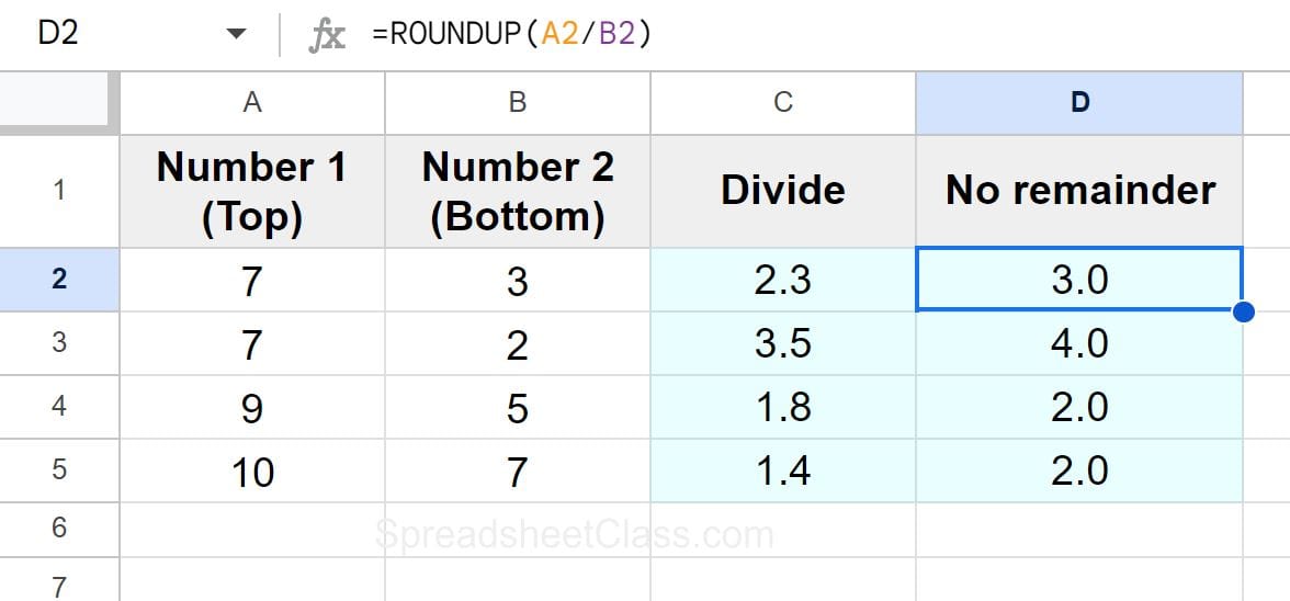
As you can see in the image above, cell D2 displays the number “3”, since the ROUNDUP function rounded up from 2.3.
The formula was copied into the cells below, and as you can see in the example image, all of the numbers were rounded up to the nearest whole number, which gives the division results without a remainder.
Note that the formula below does the same thing as the formula above, since the ROUNDUP function defaults to zero decimal places if you do not specify the number of decimal places. The formula below specifies zero decimal places, which means that the formula will round up to the nearest whole number, which is the default if no decimal places are specified at all.
=ROUNDUP(A2/B2,0)
Using the INT function to divide without a remainder
Another function that you can use to divide without a remainder, is the INT function, which rounds numbers down to the nearest integer / whole number.
We apply this formula to the division calculation in the same way that we do for the ROUND function. We simply put the division calculation inside of the INT function, like this: =INT(7/3)
This formula will give an answer of “2”, since 7/3 = 2.333 and the INT function will round down to 2.0.
=INT(7/3)
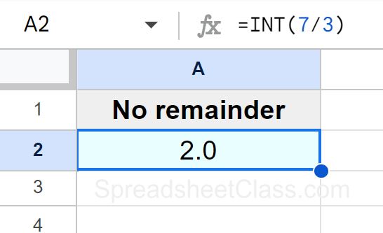
As you can see in the image above, cell A2 displays the number “2”, since the INT function rounded down from 2.3.
The Google Sheets INT function description:
Syntax:
INT(value)Formula summary: “Rounds a number down to the nearest integer that is less than or equal to it.”
Using cell references with the INT function
You can also use cell references when using the INT function.
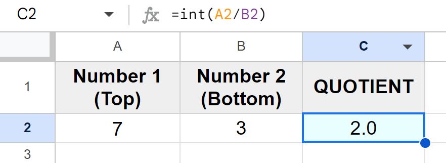
In this example, the number “7” is entered into cell A2, and the number “3” is entered into cell B2. We are going to divide cell A2 by cell B2 (A2/B2), and then apply the INT function to remove the remainder / round down to the nearest integer, like this: =INT(A2/B2)
=INT(A2/B2)
Using the QUOTIENT function to divide without a remainder
Yet another function that can be used to divide without a remainder, is the QUOTIENT function, which returns the result of one number divided by another number, but gives a whole number result.
Using this formula is slightly different from using the previous formulas. Instead of entering a division calculation and then wrapping the formula around the division calculation, this particular function both divides and rounds, so we specify the number that we are going to divide into, then type a comma, and then specify the number that we are dividing by.
In this example we are going to divide the number “7” by the number “3” by using the QUOTIENT function, and so our formula will look like this: =QUOTIENT(7,3)
This formula will give an answer of “2”, since 7/3 = 2.333 and the QUOTIENT function will round down to 2.0.
=QUOTIENT(7,3)
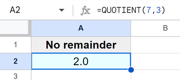
As you can see in the image above, cell A2 displays the number “2”, since the QUOTIENT function rounded down from 2.3 after dividing 7 by 3.
The Google Sheets QUOTIENT function description:
Syntax:
QUOTIENT(dividend, divisor)Formula summary: “Returns one number divided by another.”
Using cell references with the QUOTIENT function
You can also use cell references when using the QUOTIENT function.
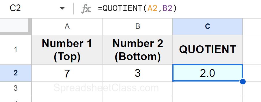
In this example we have the number “7” entered into cell A2, and the number “3” entered into cell B2. We will divide cell A2 by cell B2, and then apply the QUOTIENT function to remove the remainder, like this: =QUOTIENT(A2,B2)
=QUOTIENT(A2,B2)
Decreasing decimal places vs. rounding
It’s important to note that when using the “Decrease decimal places” option, the cell will display fewer decimal places and will round the number that is displayed in the cell, but the decimal value / remainder will still be attached to the number in the background.
Sometimes this might be exactly what you want, but if you didn’t know this it can cause confusion when a number appears to be rounded but is actually not. So if you want a number to appear rounded in the cell but still contain the decimal value / remainder when making calculations, then use the “Decrease decimal places” button, but if you want the number to be truly rounded so that the rounded number is used when you make calculations, use the formulas that we went over in this lesson, such as the ROUNDDOWN function.
Now you know the different ways to divide in Google Sheets and get a result that does not contain a remainder!