

Adding and summing are probably the most common and helpful formulas in Google Sheets. In this lesson I am going to teach you how to add and sum in a Google spreadsheet, so that you can easily add together any numbers that you want. I'll go over how to use addition to add together specific numbers and cells, and then I'll also show you how to use the SUM function to add up as many numbers as you want all at once.
I'll also show you how to use the "Explore" feature to sum numbers, which allows you to quickly sum numbers without using a formula, by simply selecting the cells that you want to sum.
To add numbers in Google Sheets, type an equals sign (=), type the first number that you want to add, type a plus sign (+), and then type the second number that you want to add, like this: =3+4 (This formula will display the number 7 in the cell that contains the formula).
You can also add cells together, which will add the numbers inside of the specified cells.
To add cells in Google Sheets, type an equals sign (=), type the first cell that you want to add, type a plus sign (+), and then type the second cell that you want to add, like this: =A1+A2 (This formula will display the number 7 in the cell that contains the formula, when the number 3 is entered into cell A1 and when the number 4 is entered into cell A2).
To sum in Google Sheets, follow these steps:
- Type "=SUM(" or click “Insert” → “Function” → “SUM”
- Type the range of cells that contain the numbers you want to sum, such as "A1:A"
- Press "Enter" on the keyboard, and Google Sheets will sum the specified range, with a SUM formula that looks like this: =SUM(A1:A)
Further below are detailed examples of how to add and sum in a variety of ways.
Using mathematical operators to add in Google Sheets
First, we will start with the most basic and common way of adding in Google Sheets, which is by using the plus sign (+), which is a mathematical operator.
In Google Sheets, the four major mathematical operators that you can use to do math, are as follows:
- Addition: Plus sign (+)
- Subtraction: Minus sign (-)
- Multiplication: Asterisk (*)
- Division: Forward slash (/)
Click here if you want to learn how to do every different kind of math in Google Sheets. In this article we will stick to using addition as well as the SUM function.
Add numbers in Google Sheets
The most simple addition formula, adds one number to another number, where the numbers are typed directly into the formula. For example, if you wanted to add the numbers 1 and 2 together, you would simply enter the formula shown below into a spreadsheet cell.
=1+2
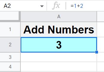
After entering the formula above, your spreadsheet will display the number 3 in the cell that contains the addition formula.
Add cells together in Google Sheets
You can also use cell references to add in Google Sheets, which means that you can tell Google Sheets to add the number, in one cell, to a number in another cell.
This makes it easy to change the numbers that you are adding by editing the numbers in the cells, without needing to modify the formula each time you want to change the numbers.
For example, if you enter the number 1 into cell A3, and you enter the number 2 into cell A4, you can add together cells A3 and A4, which will add the numbers that are entered inside them (1+2 = 3).
When specifying a cell, simply type the cell's address, which is the letter of the column that the cell is in, followed by the number of the row that the cell is in. So if the cell is in column A and in row 3, the cell's address is written as A3.
=A3+A4
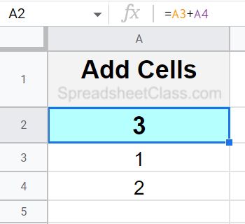
As you can see in the image above, when you add cells A3 and A4 together, the formula in cell A2 displays the number 3 (Because cell A3 has the number 1 entered into it, and cell A4 has the number 2 entered into it, and 1+2=3).
This content was originally created by Corey Bustos / SpreadsheetClass.com
Using the ADD function
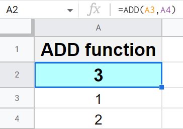
If you want, you can add by using the ADD function. This method is not as common as using the plus sign for adding. To use the ADD function, simply enter the cells that you want to add in the ADD function criteria, separated by commas, as shown below.
You can also use cell references with the ADD function, such as this example which adds together the same cells (which have the same numbers in them) as in the last example.
=ADD(A3,A4)
Adding more than two cells together
You can use the plus sign and other mathematical operators to add together as many cells as you want, as shown below. Simply enter a cell or number, type a plus sign, enter another cell or number, and repeat the process until you are adding all of the cells / numbers that you want.
However, if you are adding together numbers that are in a column or a row, like in this example, it is easier to use the SUM function, which I will go over further below.
=A3+A4+A5+A6+A7+A8
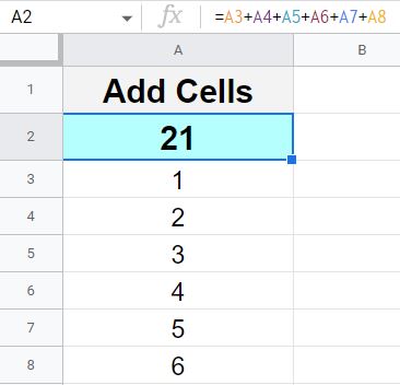
As you can see in the image above, cells A3 through A8 are all being added together with an addition formula, where each individual cell reference is added one at a time. Again, the SUM function will help you quickly add numbers in columns / rows. See further below for how to use the SUM function.
Adding non-adjacent cells
Using the plus sign to add in a spreadsheet comes in very handy when you want to add together cells that are not right next to each other (non-adjacent cells). As shown below, you can add together any cells that you need in the spreadsheet, even if the cells are not in the same row / column, and even if the cells are far apart.
=B3+C4+D5+E6+F7+G8
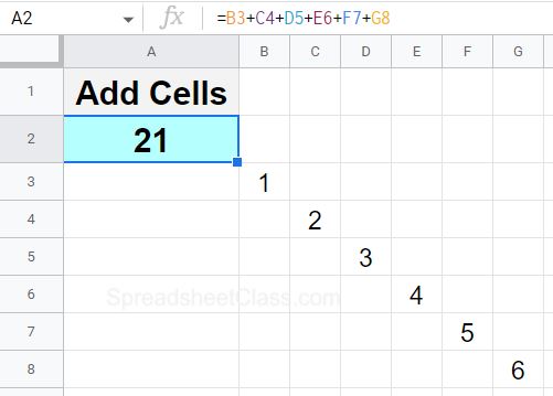
As you can see in the image above, the non-adjacent cells are being added together, where the values from cells that are not in the same column / row are being added by using the plus sign.
Using the SUM function to sum in Google Sheets
Now let's go over how to use the SUM function, which will allow you to quickly sum (i.e. "add up") many cells / numbers at once.
In the example with the SUM function, notice that I have entered the formulas at the top of the sheet. Doing this allows the formula to remain in one place as new data is added at the bottom of the sheet… so that the formula does not get in the way of new rows / data that you want to add.
If you want, you can put the SUM formula at the bottom of your data, but when you want to add new data / new rows of data to your sheet, you will have to move the SUM formula downwards to give more space for the data.
Putting the formula at the top of the sheet also allows the specified range of cells to remain the same as new data is added at the bottom, since you can set the formula to sum the entire column below it.
Click here to read more about a "Circular Dependency Error", which is when the cell that your formula is in, is within the range that the formula refers to.
Sum a column
First, let's start with the most common use of the SUM function, which is to sum a column, or in other words to sum the numbers in a column. We will use a very basic example and then later we will go over examples with real-world data.
To sum a column in Google Sheets, follow these steps:
- Type =SUM(
- Then type the range of the cells / column that contain the numbers to be summed, like this: A3:A
- Press "Enter" on the keyboard, and the cell with the SUM function will display the sum of all the numbers in the range / column that you specified. Your final formula will look like this: =SUM(A3:A)
In this example, we will sum a column of numbers, with the SUM function entered into a cell that is above the numbers to be summed. The numbers to be summed are in column A, starting at row 3.
The formula below is entered into cell A2, for this example.
=sum(A3:A)
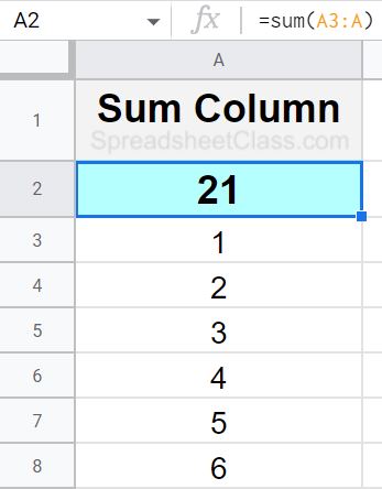
Notice that in the example image / formula above, there are numbers entered into column A, starting at row 3.
The SUM formula in cell A2 is summing / adding up all of the numbers in column A, starting from row 3, and the total of all the numbers added together is 21. Note how much easier the SUM function makes it to add up multiple numbers / cells.
If you want to sum all of the numbers to the end of a column, no matter how many rows there are, do not include an ending row in the sum range, as shown in the example formula above.
If you sum range A3:A100, the SUM function will sum the numbers in column A, in rows 3 through 100. But if you sum the range A3:A, the SUM function will sum all of the numbers in column A, starting at row 3.
Sum a row
You can also use the SUM function to sum a row of data, instead of a column (horizontal instead of vertical).
To sum a row in Google Sheets, follow these steps:
- Type =SUM(
- Then type the range of the cells / row that contain the numbers to be summed, like this: C1:1
- Press "Enter" on the keyboard, and the cell with the SUM function will display the sum of all the numbers in the range / row that you specified. Your final formula will look like this: =SUM(C1:1)
In this example we will sum a row of numbers, with the SUM function entered into a cell that is on the left of the numbers to be summed. The numbers to be summed are in row 1, starting at column C.
The formula below is entered into cell B1, for this example.
=sum(C1:1)
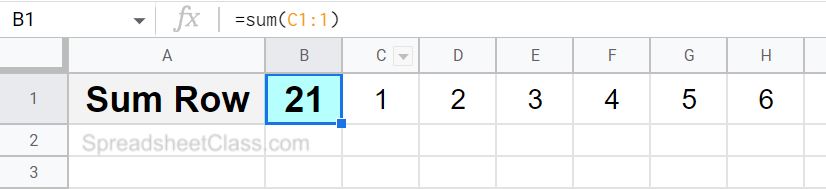
As you can see in the image above, the formula in cell B2 is summing all of the numbers in row 1, starting at column C, and the total / sum is 21.
Notice that in the example formula above, the range which represents a row, ends with a number, instead of a letter.
This is because we are indicating that the range is a row, and not a column. If you want, you could indicate an ending column like this: C1:Z1, but if you do not include a column letter in the last part of the range (after the colon), the range will refer to the rest of the row / the formula will calculate until the end of the row, like this: C1:1
Sum data with a real world example (Revenue)
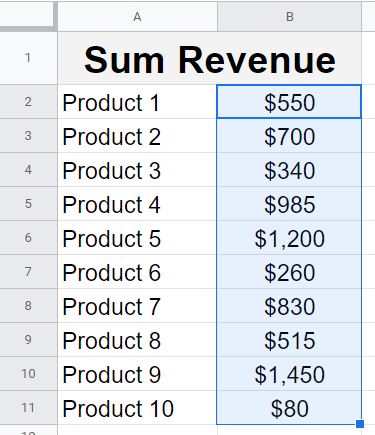
Now let's go over an example of summing with real-world example data. Below is a list of products in column A, and the revenue earned from each product listed in column B. We are going to sum the revenue from all of the products, to find the total revenue earned with all products combined.
The formula below, is entered into cell B2 for this example.
=sum(B3:B)
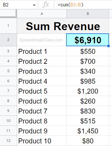
As you can see in the image above, the total revenue earned with all products combined, was $6,910.
Using the "Explore" feature to sum data quickly
Google Sheets has a unique feature that allows you to make fast calculations without a formula, by simply selecting the cells that contain the data to be calculated and looking on the bottom right of the screen.
This feature is called "Explore". For example, you can use the Google Sheets Explore feature to quickly sum numbers. This is demonstrated below.
On the bottom right of your spreadsheet, you'll notice a button that says "Explore". When you select multiple cells with numbers in them, you'll see a menu pop up near the "Explore" button, which will show the sum of the selected numbers by default… but you can also click this menu to select other types of calculations such as averaging.
For this example will use the same product revenue data from the last example, but instead of using a formula to sum the total revenue, we will use the "Explore" feature.
To sum with the "Explore" feature in Google Sheets, follow these steps:
- Select the cells / range of cells to be summed
- Look in the bottom right of your Google spreadsheet, and the sum of the selected cells / numbers will be displayed by default
- Click the menu on the bottom right where the calculation is shown, to choose other types of calculations
Step 1: Select the cells that contain the data to be summed
Step 2: On the bottom right, click the menu to the left of the "Explore" button, and choose the desired calculation, such as "Sum".
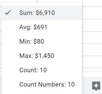
Step 3: View the calculated total / sum of the selected cells, which is displayed in the bottom right of the spreadsheet.

Sum multiple columns or sum a table of data
If you want, you can use the SUM function to sum more than one column of data, or more than one row of data. In other words you can sum an entire table of data with the SUM function.
To do this, simply type the range of cells that you want to sum, as is shown in the example below, where columns B through F are being summed by specifying the range B3:F in the SUM formula.
To sum multiple columns of data in Google Sheets, follow these steps:
- Type =SUM( to begin the sum formula
- Type the range of cells that you want to sum, such as "B3:F" (Notice that this range refers to multiple columns)
- Press "Enter" on the keyboard, and the sum of the entire range (including the values from any / all columns included) will be displayed in the cell that contains the sum formula. The final formula will look like this: =SUM(B3:F)
In this example, there are 5 days / 5 columns or revenue entered for each product, and we are going to find the sum / total of all the revenue earned, for all products, for all 5 days.
The formula below, is entered into cell A2 for this example. The data to be summed is entered in columns B through F, starting at row 3.
=sum(B3:F)
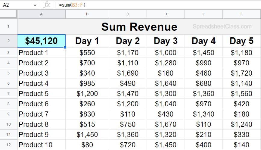
As you can see in the image above, the formula in cell A2 shows the sum of the revenue from multiple columns.
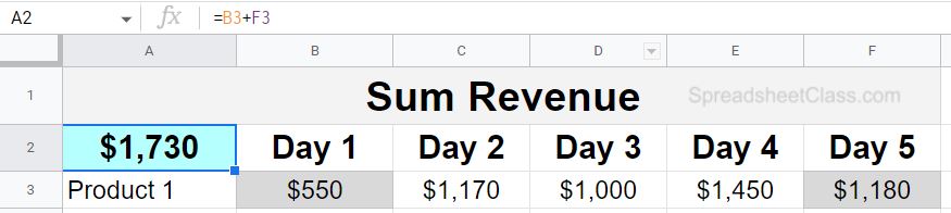
Adding non adjacent cells (Real world example)
Let's go over a quick example of adding non-adjacent cells, with realistic data.
For example, if we wanted to add the revenue earned for product 1 on day 1, to the revenue earned for product 1 on day 5, we would simply add together the appropriate cells, which in this case are cells B3 and F3. The formula and image below shows how to do this.
=B3+F3
Sum if not blank
Note that the SUM function already sums cells that are not blank by default. Blank cells are considered as a zero value, and so blank cells will not affect the SUM formula… i.e. the SUM function already "Sums if not blank".
The Google Sheets SUM formula:
Below is a diagram that shows how the SUM function works.
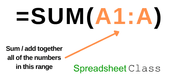
As you can see, to use the SUM function all you need to do is to specify the range of cells that contain the numbers you want to sum, and the SUM function will automatically sum / add up all of the numbers that are in the range that you specified.
The Google Sheets SUM function description:
Syntax:
SUM(A2:A100, 101)Formula summary: “Returns the sum of a series of numbers and/or cells.”
Addition formula in Google Sheets:
Below is a diagram that shows how addition formulas work in Google Sheets.
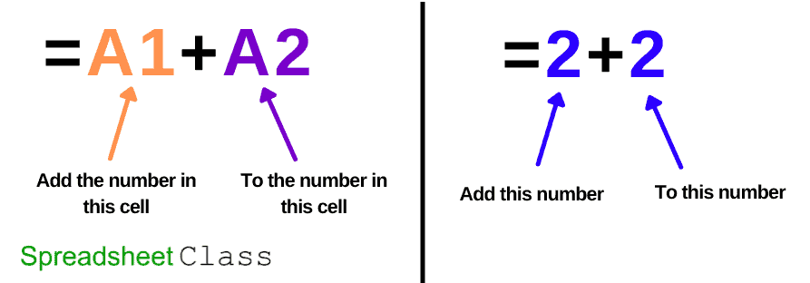
As you can see, you can use the plus sign to add together numbers, or you can also add together cells (the numbers within them), or you can use a combination of the two. For example you could type a formula like =A1 +2, which would add 2 to the number that is inside cell A1.
How I use the SUM formula and addition at my job
These formulas are very common and very useful, and I find myself using them all the time in my work.
For addition, I use this when I need to add a small amount of number together, especially of course when those numbers are not right beside each other in the spreadsheet, such as when I add the number of active courses that a student has to the number of completed courses that they have.
I use the SUM formula to do things like adding total time worked on each day, at the top of the sheet.
Pop Quiz: Test your knowledge
Answer the questions below about addition and the SUM function, to refine your knowledge! Scroll to the very bottom to find the answers to the quiz.
Question #1
Which of the following formulas adds two numbers (not cells) together?
- =A1+B1
- =2+3
Question #2
Which of these functions adds cells / cell references?
- =7+10
- =B11+B12+B13
Question #3
True or False: The SUM formula makes it easy to add many numbers together at once.
- True
- False
Question #4
Which of the following formulas would give an answer / result of 7, if the number 4 is entered into cell A1, and the number 3 is entered into cell A2?
- =4+3
- =A1+A2
- =ADD(A1,A2)
- =SUM(A1:A2)
- All of the above
Question #5
Which of the following formulas sums multiple columns?
- =SUM(A1:A)
- =SUM(A1:B)
Click here to get your free Google Sheets cheat sheet
Answers to the questions above:
Question 1: 2
Question 2: 2
Question 3: 1
Question 4: 5
Question 5: 2