

Do you have numbers in a Google spreadsheet that you want to average? This lesson will teach you multiple ways to average in Google Sheets. I will show you how to use the AVERAGE function, and I'll also show you how to average by using the SUM function with division. I'll also show you the "Explore" feature which allows you to quickly average numbers without a formula, by simply selecting the cells that you want to average.
To average in Google Sheets, follow these steps:
- Type "=AVERAGE(" or click “Insert” → “Function” → “AVERAGE”
- Type the range of cells that contain the numbers that you want to average, such as "A1:A"
- Press "Enter" on the keyboard. The final formula looks like this: =AVERAGE(A1:A)
- To average multiple cells, type each reference separated by commas, like this: =AVERAGE(A1,A2,A3)
To average by using the SUM function and division in Google Sheets, follow these steps:
- Use addition or the SUM function to add up all of the values that you want to average. If there are two students in a class, where one student earned 10 points, and the other student earned 20 points, then the total of these two values would be 30 points.
- Divide the total from the previous step, by the number of values / entries that there are. Following the same example, if there are two students, this means that we divide the total number of points (30) by the number of students (2). 30/2 = 15 So the average points earned for each student is 15. You can count the number of entries manually and then divide by a specified number, or you can use the COUNTIF function to automatically count the number of values
Click here to get your Google Sheets cheat sheet
In general, to find the average of multiple numbers, add up (or sum) all of the numbers to be averaged, and then divide the total by how many numbers / values there were.
Both of the methods above are taught in detail, in the examples further below.
Click here if you want to learn more about adding and summing in Google Sheets.
Further below are detailed examples of how to average in a variety of ways.
Using the AVERAGE function to average in Google Sheets
First, let's go over how to use the AVERAGE function to average, which is the method that is most commonly used and will allow you to set up a formula that constantly displays the average. Later I'll show you alternate ways to average in Google Sheets.
First, notice that in the examples in this lesson, the AVERAGE formulas are entered at the top of the column. Doing this will allow you to continue adding data / entries on the bottom of the sheet, without interfering with your AVERAGE formula. If you want you can put the AVERAGE formula at the bottom of your data, but if you want to add more data at the bottom of the sheet you'll need to move your AVERAGE formula downwards to allow for more space.
Note that when you put your AVERAGE function at the top of the sheet, this also allows you to set the formula to average the entire column below the formula, which means that you will not need to edit the formula range when you add new data.
Click here to learn more about "Circular Dependency Errors", which is when the cell that your formula is inside of, is within the range that the formula refers to.
Average a column
We'll start with the most common application of the AVERAGE function, which is to average a column in your spreadsheet.
To average a column in Google Sheets, follow these steps:
- Type =AVERAGE(
- Then type the range of the cells / column that contain the numbers to be averaged
- Press "Enter" on the keyboard, and the cell with the AVERAGE function will display the average of all the numbers in the range / column that you specified. Your final formula will look like this: =AVERAGE(A3:A)
In this example, we will average a column of numbers, with the AVERAGE function entered into a cell that is above the numbers to be averaged. The numbers to be averaged are in column A, starting at row 3.
The formula below is entered into cell A2 for this example.
=AVERAGE(A3:A)
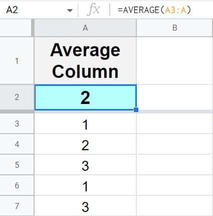
As you can see in the example image / formula above, there are numbers entered into column A, starting at row 3. The AVERAGE formula in cell A2 is averaging all of the numbers in column A, starting from row 3, and the average of all the numbers is 2.
If you want to average all of the numbers to the end of a specified column, no matter how many rows there are… do not include an ending row in the range of your AVERAGE formula (as shown in the example formula above). If you average the range C3:C100, the AVERAGE function will average the numbers in column C, in rows 3 through 100. But if you average the range C3:C, the AVERAGE function will average all of the numbers in column C, starting at row 3.
Average a row
You can also use the AVERAGE function to average a row of data, instead of a column (horizontal instead of vertical).
To average a row in Google Sheets, follow these steps:
- Type =AVERAGE(
- Then type the range of the cells / row that contain the numbers to be averaged, like this: B2:2
- Press "Enter" on the keyboard, and the cell with the AVERAGE function will display the average of all the numbers in the range / row that you specified. Your final formula will look like this: =AVERAGE(B2:2)
In this example we will average a row of numbers, with the AVERAGE function entered into a cell that is on the left of the numbers to be averaged. The numbers to be averaged are in row 2, starting at column B.
The formula below is entered into cell A2 for this example.
=AVERAGE(B2:2)
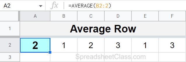
As you can see in the image above, the formula in cell A2 is summing all of the numbers in row 2, starting at column A, and the average is 2.
Notice that in the example / formula above, the range that represents a row ends with a number, instead of a letter. This is because the range represents a row, and not a column. If you want, you could indicate an ending column like this: B2:Z2, but if you do not specify a column letter in the last part of the range (after the colon), the range will refer to the rest of the row / the formula will calculate until the end of the row, like this: B2:2
Average numbers
The average function can also be used to average numbers, where you enter each specific number that you want to average directly into the formula, where the numbers to be averaged are separated by commas, as shown below.
=AVERAGE(1,2,3)
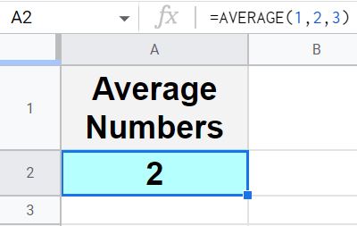
Notice in the image above that the numbers 1, 2, and 3 are being averaged, which gives an answer / result of 2 in the cell that the AVERAGE formula is entered into.
Average cells
Another way to use the AVERAGE function, is to average individual / specific cells, instead of a range of cells. This is done by entering the addresses of the cells that you want to average, separated by commas, as shown in the example formula / image below.
When you are specifying a cell / cell address in a formula, simply type the "address" of the cell, which is the letter of the column that the cell is in, followed by the number of the column that the cell is in. So if the cell is in column A and in row 5, the cell's address would be A5.
In this example we will average the numbers that are entered into cells A3, A4, and A5 (Numbers 1, 2, and 3).
The formula below is entered into cell A2 for this example.
=AVERAGE(A3,A4,A5)
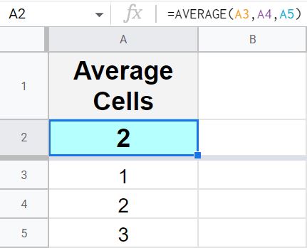
Notice in the example image above, the formula in cell A2 is averaging the numbers that are entered into cells A3, A4, and A5, which gives an answer / result of 2.
How to average by using mathematics
If you want, you can use mathematics to average in Google Sheets, where instead of using the AVERAGE function, you can add up / sum the numbers and then divide by how many values / numbers there are. See the top of this page for a very basic explanation / example of how averaging works in general.
But as a very quick review, remember that to average numbers means to add them all up and then divide by how many numbers there are. Below are several different ways of averaging without the AVERAGE function.
Click here if you want to learn how to do every different kind of math in Google Sheets.
In the following two examples the number to divide by (how many values / numbers there are) is being manually entered into the formula itself. Later I will show you how to use the COUNTIF function to automatically count how many numbers there are, but let's keep it basic for now.
Using the SUM function with division to average
The easiest way to add up a large amount of numbers is to use the SUM function. In this example, we are going to use the SUM function to add up 5 numbers, and then we will divide by 5 to get the average.
The numbers to be averaged are entered into column A, starting at row 3… and there are 5 numbers to be averaged.
The formula below is entered into cell A2 for this example.
=sum(A3:A)/5
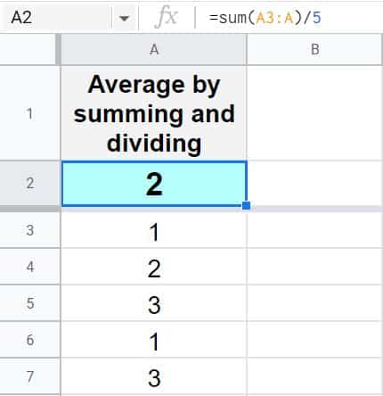
Notice in the example image above, the formula in cell A2 is adding up / summing all the numbers in column A (starting at row 3), and then dividing by 5, which gives an average of 2. (1+2+3+1+3=10 and 10/5=2)
Using addition and division to average
Let's go over a quick example that is similar to the previous example, but instead of using the SUM function to add up the numbers, we will use addition to add up the numbers. We will use a plus sign to add the cells that contain the numbers to be averaged, and then we will divide the total by how many numbers there are.
The same numbers to be averaged are entered into column A, starting at row 3 (5 numbers to be averaged).
The formula below is entered into cell A2 for this example.
=(A3+A4+A5+A6+A7)/5
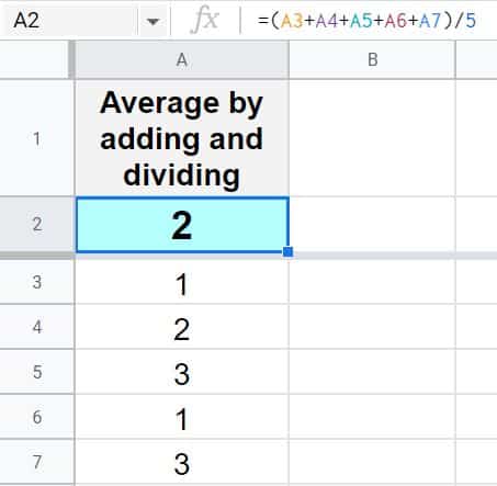
Notice that the formula above uses the plus sign instead of the SUM function to add up the numbers, and then the total is divided by 5, which gives an answer / average of 2. (1+2+3+1+3=10 and 10/5=2)
Average percentages with the AVERAGE function
Now let's go over an example with real-world data. In this example, we will average the percentages of student test scores.
Percentages are simply numbers that are displayed differently (with a percentage symbol), and so averaging percentages in a spreadsheet is done in the same way that averaging numbers is.
To average percentages in Google Sheets, follow these steps:
- Type =AVERAGE( in a spreadsheet cell
- Type the range of cells that contains the numbers / percentages to be averaged, like this: B3:B
- Press "Enter" on the keyboard, and the cell with the AVERAGE formula will display the average of the percentages that are in the specified range. The final formula will look like this: =AVERAGE(B3:B)
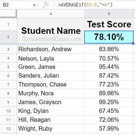
The student names are in column A, and the test scores to be averaged are in column B (starting at row 3).
The formula below is entered into cell B2 for this example.
=AVERAGE(B3:B)
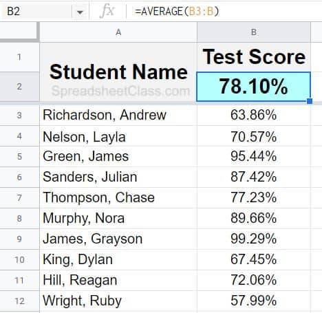
Notice in the example image above, the average percentage of all the student test scores, is 78.10%.
Using the "Explore" feature to average data quickly
Google Sheets has a very useful tool that allows you to make quick calculations without using a formula… by simply selecting the cells that contain the data to be calculated, and viewing the calculated number on the bottom right of the screen. This feature is called "Explore". For example, you can use the Google Sheets Explore feature to quickly average numbers. This feature is shown below.
On the bottom right of your Google spreadsheet, you'll notice a button that says "Explore". If you select multiple cells that have numbers inside of them, you'll see another menu pop up near the "Explore" button, which will show the sum of the selected numbers by default… but you can also click this menu to select other types of calculations.
For this example will use the same student test score data from the last example, but instead of using a formula to average the test scores, we will use the "Explore" feature to average.
To average with the "Explore" feature in Google Sheets, follow these steps:
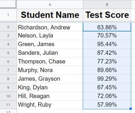
- Select the cells / range of cells to be averaged
- Click the menu on the bottom right where the calculation is shown, and click "Avg:" which stands for "Average"
- Look at the bottom right of the screen, and the automatically calculated average of the selected cells will be displayed
Step 1: Select the cells that contain the data to be averaged
Step 2: On the bottom right, click the menu that is to the left of the "Explore" button, and choose the desired calculation, such as "Average".
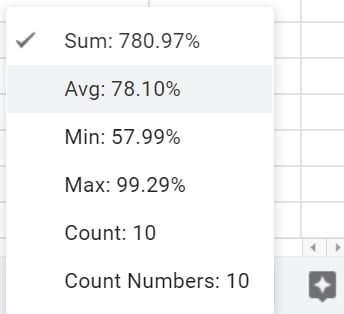
Step 3: View the average of the selected cells, which will be displayed on the bottom right of the spreadsheet.

Average multiple columns or average an entire table of data
You can also use the AVERAGE function to average multiple columns of data (or multiple rows of data). This means that you can average an entire table of data with the AVERAGE function, if you want. To do this, simply type the range of cells that you want to average, as shown in the example below… where columns A through C are being averaged by specifying the range A3:C in the AVERAGE formula.
To average multiple columns of data in Google Sheets, follow these steps:
- Type =AVERAGE( to begin the average formula
- Type the range of cells that you want to average, such as A3:C (Notice that this range refers to multiple columns of data)
- Press "Enter" on the keyboard, and the average of the entire range (including the values from any / all columns included) will be displayed in the cell that contains the average formula. The final formula will look like this: =AVERAGE(A3:C)
In this example we have three columns of numbers, and we are going to find the average of all of the numbers, from all 3 columns.
The formula below, is entered into cell A2 for this example. The data to be averaged is entered in columns A through C, starting at row 3.
=AVERAGE(A3:C)
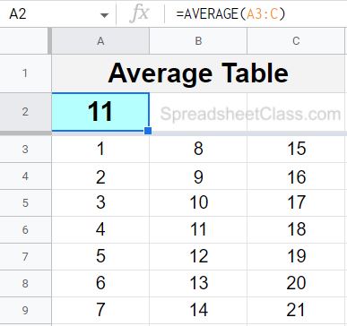
Notice in the image above, that the formula in cell A2 shows the average of the numbers that were entered into multiple columns.
Average by using COUNTIF, SUM, and division
Earlier we went over examples of how to use mathematics to average without using the AVERAGE function, where the number to divide by (how many values / numbers there are) was entered directly into the formula. But now let's go over an example of automatically counting how many numbers there are, so that you do not have to directly enter the number to divide by in the formula.
We will do this by using the COUNTIF function (counts where specified criteria is met), to count how many non-blank cells that there are, which in this case tells us how many numbers there are in the list of numbers to be averaged. We will use the same student test score data from the previous examples.
To count non-blank cells in Google Sheets, follow these steps:
- Type =COUNTIF( into a spreadsheet cell
- Type the range of cells that you want to count / consider for the function, like this: A3:A
- Type a comma, and then enter the following characters / symbol, which represents the logic "not blank": "<>"
- Press "Enter" on the keyboard, and the cell that contains the formula will show the number of non-blank cells in the range that you specified. The final formula will look like this =COUNTIF(A3:A,"<>")
The symbol <> ("less than" sign followed by a "greater than" sign) means "Not Equal" in Google Sheets. When used in the COUNTIF function, and entered between quotation marks, the characters / symbol "<>" is interpreted by Google Sheets as "Not Blank" or "Not Empty". In some other formulas, such as the FILTER function, the "Not Equal" symbol will come before the quotation marks, like this <>"". But again with the COUNTIF function the "Not Equal" symbol goes inside the quotation marks when counting non-blank cells.
After following the steps above, you know how to count non-blank cells… and now you can use the COUNTIF function as a reference for the number of values to divide by / to be averaged, when calculating averages in a spreadsheet without the AVERAGE function (as demonstrated below).
The first formula counts the number of cells in column A that are not blank, and the second formula does the averaging (while referring to the cell with the COUNTIF formula to specify the number to divide by)
The COUNTIF formula directly below, is entered into cell A2 for this example.
=COUNTIF(A3:A,"<>")
The formula directly below, is entered into cell B2 for this example.
=sum(B3:B)/A2
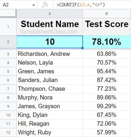
Notice in the example image / formulas above, that the COUNTIF function in cell A2 counts the number of non-blank cells, which in this case is 10… meaning that there are 10 numbers to be averaged in column A… and therefore the number that we want to divide by when averaging, is 10.
Then the formula in cell B2 sums the numbers, and then divides by cell A2 (the cell that the COUNTIF function is in). The combination of these two formulas finds the average of the numbers in the specified range, where the number of values to average / divide by is automatically calculated.
If you want, these formulas could be combined into a single formula, like this: =sum(B3:B)/COUNTIF(A3:A,"<>")
In the combined formula above, instead of putting the COUNTIF function in its own cell, and then referring to that cell with the other formula… we simply entered the COUNTIF function directly into the same formula, in the denominator.
Average across sheets
If you have numbers on different spreadsheets that you want to average, you can easily do this.
To average across multiple sheets in Google Sheets, you will need to specify tab names when referring to the data to be averaged. When referring to data on another tab in Google Sheets, before typing the range or cells address, include the name of the tab followed by an exclamation point, like this: Sheet1!A2
Note that is there is a space in the tab name, you will need to put an apostrophe before and after the tab name, like this: 'Sheet 1'!A2
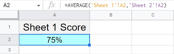
In this example we are going to average two different numbers that are each on a separate sheet, where the formula is on a completely different tab than the numbers to be averaged.
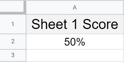
The number 0.5 (50%) is entered into cell A2 on the tab named "Sheet 1"
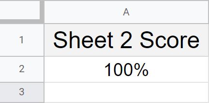
The number 1 (100%) is entered into cell A2 on the tab named "Sheet 2"
We are going to average these cells / numbers with a formula on a completely different tab, by using the formula below.
=AVERAGE('Sheet 1′!A2,'Sheet 2'!A2)
Below shows the tab that contains the average formula. Notice that the cell which contains the formula displays an average of 0.75 (75%), because 0.5 + 1 = 1.5, and 1.5 / 2 = 0.75
Below shows the number entered on sheet 1.
Below shows the number entered on sheet 2.
If you want, you can also use the AVERAGE function to average ranges of numbers across sheets, instead of just averaging individual cells across sheets. If we wanted to average column A from "Sheet 1" as well as column A from "Sheet 2", the formula would look like this: =AVERAGE('Sheet 1′!A2:A,'Sheet 2'!A2:A)
Fixing the #DIV/0! error when averaging (Divide by zero error)
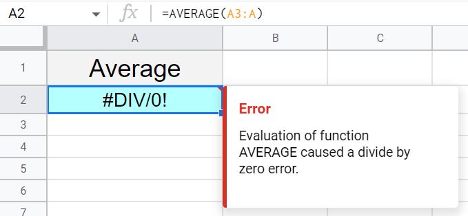
Since averaging numbers requires division, and since you cannot divide by zero…averaging in a spreadsheet may sometimes cause a "Divide by zero" error. When this happens the cell with the average formula in it will display the following error: #DIV/0!
When you hover your cursor over the cell with the divide by zero error, Google Sheets will display the following message: "Evaluation of function AVERAGE caused a divide by zero error"
If you are using a division formula, the divide by zero error message will say this: "Function DIVIDE parameter 2 cannot be zero."
This error occurs when there is no data in the range that the average function or the division formula refers to, which means that the denominator would be zero… and since it is not possible to divide by zero, this causes an error.
To fix the divide by zero error when averaging in Google Sheets, simply make sure that the cells that you are averaging are not empty.
In this example, the AVERAGE function in cell A2 is displaying a #DIV/0! error, because the function is referring to column A (starting at row 3), but there is no data in the column. After adding numbers in column A, this fixes the divide by zero error.
In other situations where you see a divide by zero error, such as when doing division, remember that the error is because the formula is trying to divide by zero. With this knowledge you can investigate the error to find why the denominator is zero in that particular case… and from there you will know how to fix the error so that you are no longer dividing by zero.
=AVERAGE(A3:A)
Average if no blank (Ignore blanks) with the AVERAGEIF function
The AVERAGE function ignores blanks by default, but in case you want to know how to build the logic into the formula despite the default behavior, here is how to write a formula that tells Google Sheets to ignore blanks. In the next example we will make a very slight change to the formula to make the AVERAGE function ignore zeros, but for now we will go over averaging non-blank cells.
To do this we will use the "Not Equal" symbol again (<>), with a formula called AVERAGEIF, which averages numbers where a specified criteria is met. In this case we are going to use the AVERAGEIF function to tell Google Sheets to average column B (starting at row 3), where column B is not blank.
Refer to the example above with the COUNTIF function to read more about using the "Not Equal" symbol in Google Sheets.
The AVERAGEIF function will allow you to include an optional "Average Range" if you want to average a column other that the criteria column… but in this case our criteria range is the same as the average range, and so we will leave out the average range, and Google Sheets will default the average range to the criteria range.
Again we will use the same student test score data. You will notice that the answer in this example is the same answer from the previous examples with this data, and that's because the AVERAGE function defaults to ignoring blank cells anyways.
The formula below is entered into cell B2 for this example. The numbers to be averaged are in column B, starting at row 3.
=AVERAGEif(B3:B,"<>")
The formula directly below will do the same thing as the formula above, because the AVERAGE function ignores blanks by default.
=AVERAGE(B3:B)
Notice that the AVERAGEIF function refers to cells all the way to the bottom of column B, and even though the data only extends to row 12, the formula is ignoring the blank cells and only averaging the cells that have numbers in them.
This content was originally created by Corey Bustos / SpreadsheetClass.com
Average if not zero (Ignore zeros)
When averaging in a spreadsheet, you will sometimes want to find the average of a list of numbers, where you want to ignore the zeros. This can be done with the same method that we used in the last example, where we used the AVERAGEIF function, and the "Not Equal" symbol. Except in this case, instead of telling Google Sheets to ignore blanks, we are going to tell Google Sheets to ignore zeros when we average.
To do this we will use the following criteria with the AVERAGEIF function, which means "Not equal to 0": <>0
The data that we are using is similar to the previous examples, but this time there are 5 student scores that are 0%. Our formula is going to average all of the numbers except for zeros, so that we can find the class average among students who do not have a zero.
Again, see the previous example to learn more about the AVERAGEIF function, and see the example with the COUNTIF function to learn more about the "Not Equal" symbol.
The formula below is entered into cell B2 for this example. The data to be averaged is in column B (starting at row 3).
=AVERAGEIF(B3:B,"<>0″)
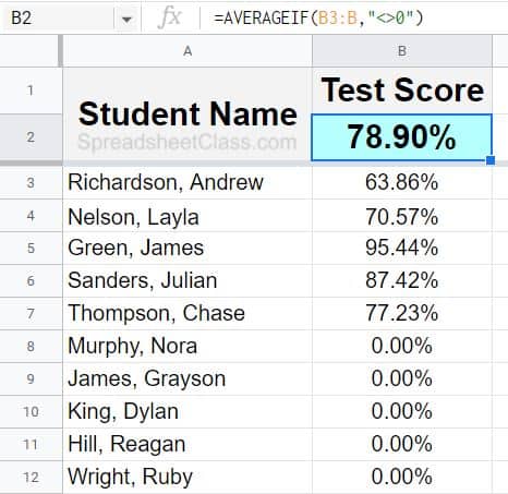
Notice in the example image above, that even though 5 students have a score of 0% (half of the class), the AVERAGEIF formula is still showing an average of 78.9%, because it is ignoring the zeros, and only averaging the numbers that are not zero (If we did not ignore the zeros in this case, while using a normal AVERAGE function, the average would have been much lower as the zero scores would have brought the average down.
The Google Sheets AVERAGE formula:
Below is a diagram that shows how the AVERAGE function works.
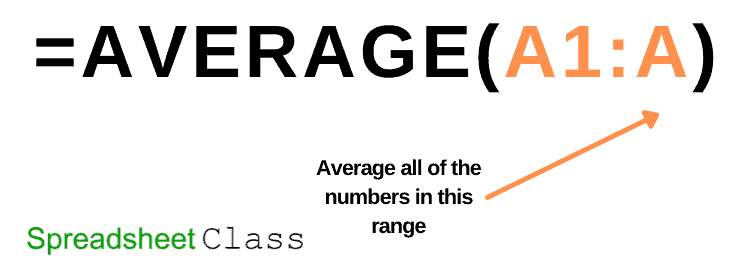
As you can see, all you have to do is specify a range of cells that you want to average, and the AVERAGE function will automatically average the numbers that are in the specified range.
The Google Sheets AVERAGE function description:
Syntax:
AVERAGE(A2:A100, B2:B100)Formula summary: “Returns the numerical average value in a dataset, ignoring text.”
How I use the AVERAGE formula at my job
As a data specialist at an online school, I use the AVERAGE formula to do things like calculating the average grade for each student, or the average for each location, or each course. There are lots of different averages to calculate when it comes to student data.
Pop Quiz: Test your knowledge
Answer the questions below about averaging in Google Sheets, to refine your knowledge! Scroll to the very bottom to find the answers to the quiz.
Click here to get your Google Sheets cheat sheet
Question #1
Which of the following formulas will average a column?
- =AVERAGE(A1:A)
- =AVERAGE(A1:1)
Question #2
Which of these functions will average a row?
- =AVERAGE(A1:A)
- =AVERAGE(A1:1)
Question #3
True or False: There are multiple ways to average in Google Sheets… but the AVERAGE function makes it easy / fast to average.
- True
- False
Question #4
Which of the following formulas will average the numbers 2 and 4 (answer of 3), if cell A1 has the number 2 entered into it, and cell A2 has the number 4 entered into it?
- =AVERAGE(2,4)
- =AVERAGE(A1,A2)
- =AVERAGE(A1:A2)
- =(2+4)/2
- =(A1+A2)/2
- All of the above
Question #5
Which of the following formulas averages multiple columns?
- =AVERAGE(A1:A)
- =AVERAGE(A1:C)
Answers to the questions above:
Question 1: 1
Question 2: 2
Question 3: 1
Question 4: 6
Question 5: 2