
When you are using formulas in Google sheets, you will often come across situations where you need to use the "not equal" sign, but not a lot of people know how to type the not equal sign or how to use it in formulas.
To type the not equal sign in Google Sheets, simply type a "less than" symbol followed by a "greater than" symbol, like this: <>
In this article I am going to show you all the different ways to use the not equal sign, from the basics of comparing cells and values, to using the not equal sign in a variety of formulas. I will also show you two functions that you can use to express "not" / "not equal".
Sometimes the not equal sign is entered inside of quotation marks in a formula, and with some formulas it is not, but I'll show you both cases in this lesson.
Use the Not Equal sign to compare values and cells
The not equal sign "<>" can be used to compare two values / two cells in Google Sheets, and determine if they are not equal to each other. This will return either TRUE or FALSE as a result, indicating whether the condition is met or not. When comparing two values / cells to check if they are NOT equal, a result of TRUE means that the values are not equal, and FALSE means that the values are equal.
Compare cells
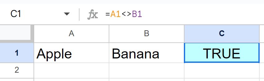
The most common use of the not equal sign is to compare cell references to check if they are not equal. For instance, if you have values in cells A1 and B1, you can use the formula =A1<>B1 to check if the values in these cells are different. If they are indeed different, the formula will return TRUE; otherwise, it will return FALSE.
In this example, cell A1 contains the word "Apple" and cell B1 contains the word "Banana"
The formula =A1<>B1 will return TRUE because "Apple" is not equal to "Banana" (as shown in the image below).
=A1<>B1
If you want you can use the equals sign to check if two cells / values are equal to each other, like this: =A1=B1
Compare text values
You can also type the text that you want to compare directly into the formula, by putting the text between quotation marks.
For example, if you want to ensure that a cell C2 doesn't contain the value "N/A" you can use the following formula: =C1<>"N/A"
Or if you want to ensure that cell B2 does not contain the text "Void", you can use the formula below:
=B2<>"Void"
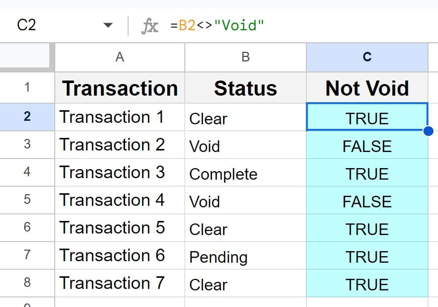
As you can see in the image above, the formula returns TRUE because it is true that cell B1 does NOT contain the word "Void".
Then this formula can be copied down the column to apply the formula to the entire column.
Using the NE function to check where not equal
If you want, you can use a function instead of an operator to express "not equal" in Google Sheets, although the operator is much easier and more common to use. The NE function is the "Not Equal" function, and allows you to check two values / cells to see if they are not equal. The function returns TRUE is the values are not equal, and returns FALSE if the values are equal.
The formula below will perform the same operation as the formula in the previous example (Checks if A1 is not equal to cell B1).
=NE(A1,B1)
The NE function can be used as an alternative for the not equal operator.
Using the NOT function to check where not equal
If you want, you can also use the NOT function, to check if values are not equal, as shown in the formula below. Again it is easier to simply use the not equal operator, and that is why we will stick to the operator method for the remaining examples.
=NOT(A1=B1)
Using the Not Equal sign to filter data with the FILTER function
When using the FILTER function you will sometimes need to filter data where a certain column is not equal to a specified criteria. You can use the not equal sign in combination with the FILTER function to filter data to show only records that do not match a specific criterion.
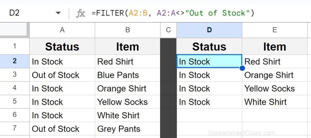
If you have a list of products in column B, and the status of the product in column A, and you want to filter out all products except those that are not equal to the status of "Out of Stock," you can use the formula below:
=FILTER(A2:B, A2:A<>"Out of Stock")
Filter where not blank using the Not Equal sign
You can also use the not equal sign to filter a data set where a specified column is not blank.
Imagine you have a dataset in columns A and B, and you want to filter out rows where the values in column A are not blank. Here's how you can do this by using the FILTER function with the not equal sign:
Column B contains the item name, and column A contains the item status. If the item is out of stock, in this example the cell is left blank in column A. We are going to tell Google Sheets to filter columns A and B, where column A is not blank. We do this by using the not equal sign followed by two quotation marks. Two quotation marks together indicate "Blank" / empty value to Google Sheets.
=FILTER(A2:B, A2:A<>"")
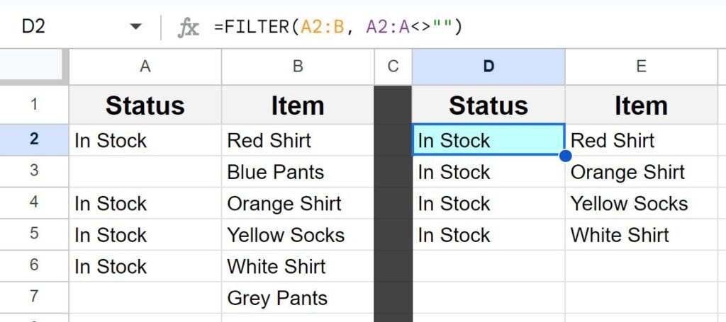
This formula instructs Google Sheets to filter columns A and B where the cells in column A are not equal to an empty value (""), denoted by the not equal sign ("<>").
As shown in the image above, the dataset now displays only the rows where column A is not blank.
In this case the items that are out of stock simply have a blank cell in column A, and so this formula that filters where column A is not blank, displays a list of items that are not out of stock, like in the last example.
Using the Not Equal sign with the COUNTIF Function
Another formula that is very useful to use with the not equal sign, is the COUNTIF function. You can count the number of cells in a range that are not equal to a specified criteria. Let's start by using text and numbers as the criteria, and then I will show you how to use cell references when the COUNTIF criteria contains an operator like the not equal sign.
Suppose you have a list of student names in column A, and test scores in column B… and you want to count the number of scores that are not equal to zero. You can use the COUNTIF function to do this:
=COUNTIF(B2:B, "<>0")
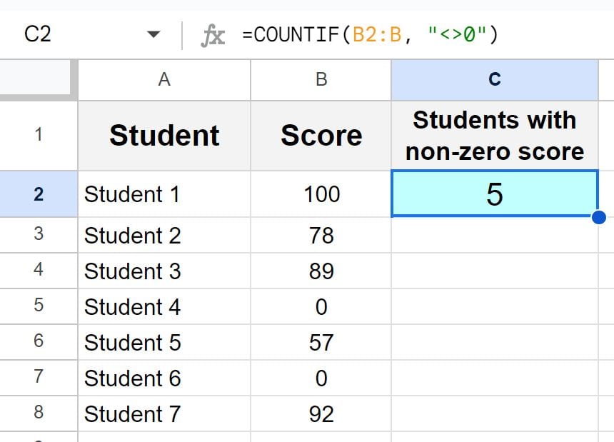
The formula above will count all the scores in column A that are not equal to 0.
Note how when using the COUNTIF function, when you use an operator like the not equal sign in the criteria, the operator / not equal sign is entered inside of quotation marks, along with the value criteria being specified, like this "<>No"
Count if not blank
You can also use the not equal sign with the COUNTIF function to count cells that are not blank. When specifying "not blank" in the COUNTIF function, we enter the not equal sign between quotation marks like this: "<>"
Suppose you have student names in column A and test scores in column B, and you want to count how many cells in column B that are not blank (i.e. how many tests have not been taken). We can do this by using the formula below:
=COUNTIF(B2:B, "<>")
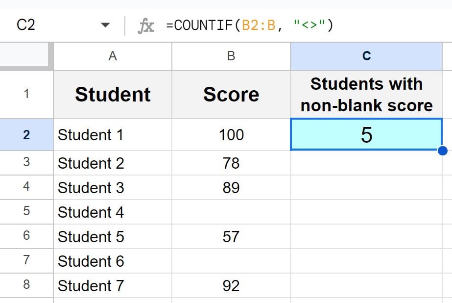
The formula above counts all the cells in column B that are not blank.
Using cell references with the COUNTIF function and the not equal sign
When you use an operator and a cell reference in the criteria for the COUNTIF function, you have to use an ampersand symbol ("&") as shown in the example below. In this case, the operator still goes between quotation marks, and then this is combined with the cell reference by using the ampersand, like this: "<>"&D1
Let's say you have a list of test scores in column B, and you want to count how many scores in that column are not equal to a specific value stored in cell D1, which is 0. Here's how you can do this by using the COUNTIF function:
=COUNTIF(B2:B, "<>"&D1)
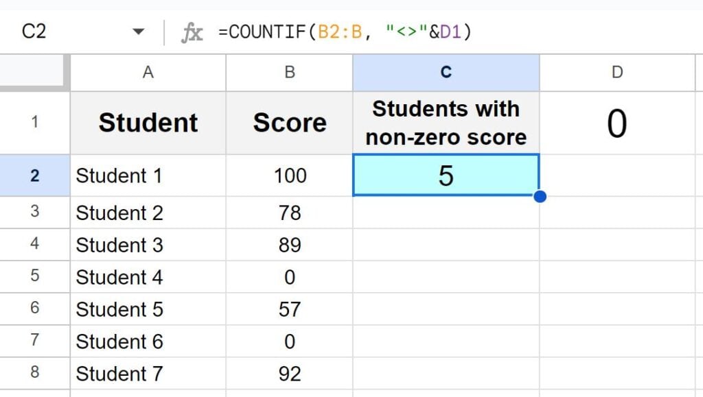
The formula above utilizes the not equal sign ("<>") to compare the values in column B with the value stored in cell D1. The ampersand symbol ("&") is used to concatenate the not equal sign with the cell reference, forming the desired criteria.
Compare SUM functions
Often, you might find yourself dealing with two sets of data in separate columns and the need to ascertain whether the sum of the values in one column is not equal to the sum in another. This can be done by using the not equal operator ("<>").
In this example, in column B we have the inventory amounts for a list of items, as stated by the computer system, and in column C we have the actual amounts counted by staff members. We want to check if the sum of the values in column B is not equal to the sum of the values in column C. To do this you can use the following formula:
=SUM(B2:B) <> SUM(C2:C)
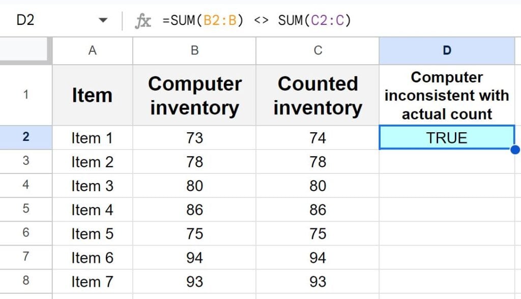
The formula above will return "TRUE" if the sum of values in column B is not equal to the sum of values in column C, and it will return "FALSE" if they are equal. As you can see in the example image, the formula has returned TRUE because the sum of each column is not equal.
Compare the cells of sum functions
If you want, instead of directly comparing two SUM functions in the same formula, you can put your SUM functions in individual cells, and then simply compare those two cells. This has the same effect, but is simply done in a different way. This is the way that I prefer to compare SUM functions.
Imagine you have two sets of data in columns B and C, and you want to determine if the total sum of values in column B is not equal to the total sum of values in column C, but you want to do it by comparing simple cell references.
First we will calculate the sum of the values in column B, in cell B2, by using the SUM function like this: =SUM(B3:B)
Then calculate the sum of the values in column C, in cell C2, by using the SUM function like this: =SUM(C3:C)
Then in cell D2, we use the not equal sign to compare the two cells / SUM functions, like in the formula below:
=B2<>C2
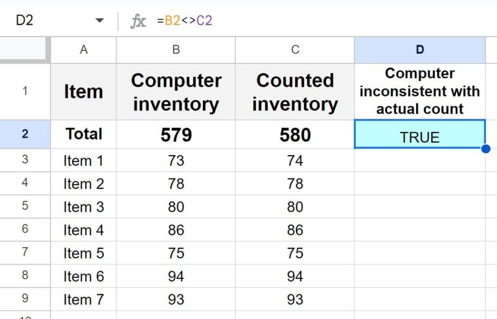
As you can see in the example image, the formula has returned TRUE because the sum of each column is not equal.
Using the not equal sign with the IF function in Google Sheets
Another formula where you can use the not equal sign, is the IF function.
To illustrate this concept, let's revisit the simple example involving apples and bananas. We will compare two cells again to check if they are not equal, but this time by using the IF function we will specify custom values to display when the criteria is met / not met.
We have two cells, A1 and B1, where A1 contains the word "Apple" and B1 contains the word "Banana." You want to create a formula that checks if these two cells are not equal, and if they are not equal / are different, we want the formula to display the words "Not Equal". If the two cells are equal, we want the formula to display the word "Equal".
You can do this using the IF function with the not equal sign as shown below:
=IF(A1<>B1, "Not Equal", "Equal")
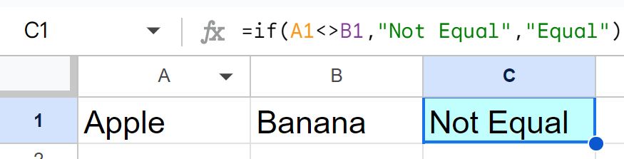
The formula above utilizes the not equal sign ("<>") within the IF function to compare the values in cells A1 and B1. If the values are not equal, it returns "Not Equal"; otherwise, it returns "Equal.
If the values in cells A1 and B1 were the same, the formula would have returned "Equal." However, because they are different, the formula returns "Not Equal."
Click here to get your Google Sheets cheat sheet
How I use the Not Equal operator in my work
At my job at an online school, I use the not equal sign to do things like filtering a list of courses where the status is not equal to "Dropped", or averaging a grade across all courses that are not "Dropped" status.