How to filter based on a list in Excel

When filtering data in Excel you may sometimes need to filter by an entire list of values, rather than by just a single/few specified values. There is a way to do this by using formulas, and it is fairly easy! You can use the FILTER and COUNTIF functions to filter based on a list in Excel.

To filter by a list in Excel, use the COUNTIF function to give an indication of whether or not each row meets your criteria, and then use the FILTER function to filter out the rows that do not meet your criteria.

There is also a way to filter by a list without using formulas, but it takes longer and is more difficult. Simply using formulas is the easiest way to filter by a list in Excel.

Here are formulas that you can use to filter by a list in Excel:

The COUNTIF and FILTER formulas below must both be used to accomplish the task of filtering by a list of items / criteria. Further below I will teach you how to use these formulas together in your sheet to file by a list.

Filter Where Found in List

• =COUNTIF(F2:F12,A3)

• =FILTER(A3:C17,D3:D17=1)

FILTER Where NOT in List

• =COUNTIF(F2:F12,A3)

• =FILTER(A3:C17,D3:D17<>1)

Filter by list from another sheet

• =COUNTIF('Tab 2'!A2:A12,A3)

• =FILTER(A3:C17,D3:D17=1)

• Alternate: =FILTER('Tab 1′!A3:C17,'Tab 1'!D3:D17=1)

In this article I will stick to using the FILTER and COUNTIF functions, since this is the faster and more reliable choice for filtering a range by an array in Excel.

This article focuses on filtering by a list in Excel, but check out this article if you want to learn how to filter by a list in Google Sheets.

If you want to learn how to use the FILTER function to perform ordinary filtering tasks, here is an article that will help you learn the FILTER function from the ground up.

But here we will only be filtering by lists/arrays/columns of data.

I have provided multiple examples showing the different ways to set up the formulas depending on how your data is arranged (i.e. depending on which tab your data/formula is on).

Filter rows based on a list in one sheet vs. multiple sheets

To start with, we will put our formula, our unfiltered data, and the list to filter by, all on the same tab so that you can easily see how the formula is set up and how it functions. But further below I will show you how to use multiple tabs while filtering by a list.

In the first examples we will start very simple, and filter a range of data, by a single-column / list, where the list that we are going to filter by does not contain any extra entries that are not present in the source data (data to be filtered).

This is not always how it will be in the real world… but this will make it easy to see what the formula is doing.

Filter a range by a list in Excel

In this example, we have a set of data that shows a list of employees within an individual department at a company, as well as their contact information. We also have another list that shows employees within the department who are eligible for a bonus.

We are going to filter the data set that shows employees and their contact information, by the list of eligible employees… so that only the contact information data of eligible employees is displayed in the filter output.

The task: Show employee contact information for employees who are eligible for a bonus

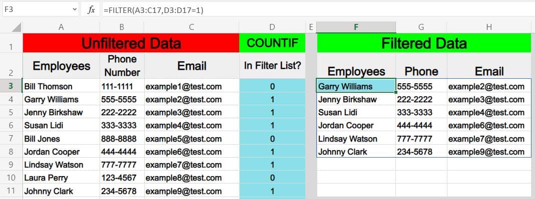
The logic: In column D, use the COUNTIF function to check whether the names in column A are contained in the list to filter by in the range F3:F17. Filter the range A3:C17, where the values in the range D3:D17 are equal to 1.

The formulas: The COUNTIF formula below, is entered in cell D3, and is copied into the cells below it to fill column D. The FILTER formula below is entered in cell H3.

=COUNTIF(F2:F12,A3)

=FILTER(A3:C17,D3:D17=1)

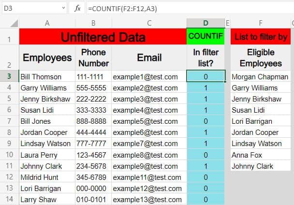
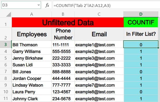
As shown in the example above, column D is being used as a place for the COUNTIF function to provide a simple indication of whether each name in column A is found within the "list to filter by" in column F.

If the name is found in the list the cell will display the number 1, and if it is not found in the list the cell will display the number 0.

This allows you to use column D as the criteria for the filter function, where you can simply tell Excel via the FILTER function to show only the rows where column D is equal to 1 (as shown below).

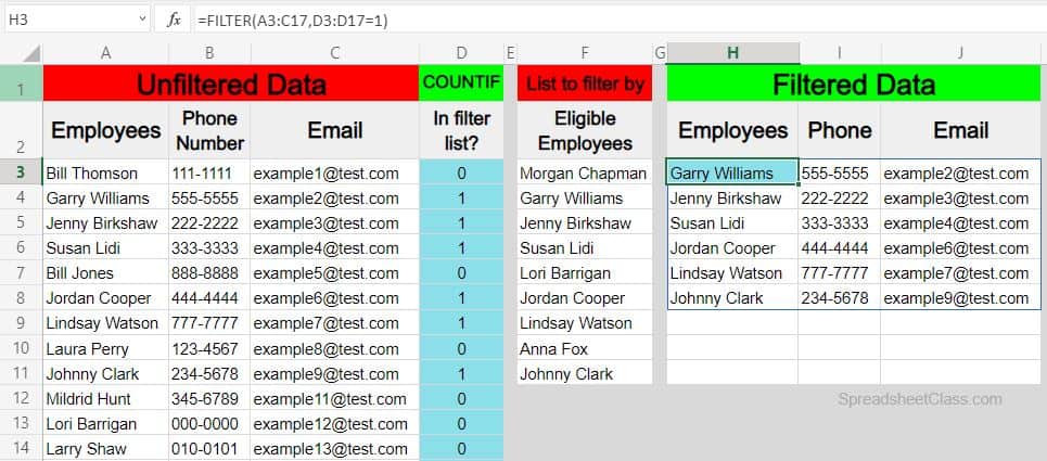
Now the filtered results in columns H through I only show the rows containing names / employees who are on the eligibility list.

Filter based on a list in Excel, where the criteria is NOT found in list

So in this example, let's say that we want to use the same data / list to filter by as the previous example, but in this case we want to show only the rows where the name is NOT in the eligibility list. In other words we will display a list of employees who are NOT eligible for a bonus.

You might have already recognized that you can do this by changing the filter criteria from "=1" to "=0". This will definitely work, but you might not always be dealing with numbers as a part of your FILTER formula criteria, and so if you ever need to filter rows where NOT equal to a certain string of text, you'll need to know how to use the "Not equal to" operator / sign in Excel.

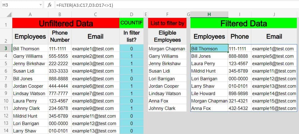
The "Not equal to" sign in Excel is expressed like this <>, which is a "less than" symbol followed by a "greater than" symbol. We will use this below to display only rows that are not equal to 1.

The task: Show employee contact information for employees who are NOT eligible for a bonus

The logic: In column D, use the COUNTIF function to check whether the names in column A are contained in the list to filter by in the range F3:F17. Filter the range A3:C17, where the values in the range D3:D17 are NOT equal to 1.

The formulas: The COUNTIF formula below, is entered in cell D3, and is copied into the cells below it to fill column D. The FILTER formula below is entered in cell H3.

=COUNTIF(F2:F12,A3)

=FILTER(A3:C17,D3:D17<>1)

Filtering by a list when the data is on separate sheets

Now that you know how to filter by a list where all of the data and the formula are held on the same sheet/tab, let's go over how to filter by a list when using multiple tabs.

There are a variety of arrangements that are possible when using multiple tabs for filtering a range by an array, and so I'll go over each of them.

In the examples below, both the unfiltered source data (data to be filtered) and the list to filter by are given in the format of multiple column ranges. In other words, the list that we want to filter by is provided with other columns of data beside it this time. This will not change how we setup the formula, but it is important to learn how to identify your column references with data that looks like this.

This type of situation where the list to filter by is attached to other data can be expected in the real world… but it presents another potentially confusing situation with setting up your formula references because of the added columns. i.e. It's easier to identify the list to filter by when the list is just a single column.

Again, if you are setting up a formula and you find yourself confused, first determine which data needs to be filtered, and which data you are using to filter with/by, then use the COUNTIF with the FILTER function as explained in this lesson.

Source data and formula on the same sheet

Here is an example showing how to set up your formula when the unfiltered source data and filter formula are on the same tab… but where your list that you want to filter by is on a separate tab.

Unfiltered source data & COUNTIF function: Tab 1

FILTER formula: Tab 1

List to filter by: Tab 2

The formulas: The COUNTIF formula below, is entered in cell D3 of Tab 1, and is copied into the cells below it to fill column D. The FILTER formula below is entered in cell F3 of Tab 1.

=COUNTIF('Tab 2'!A2:A12,A3)

=FILTER(A3:C17,D3:D17=1)

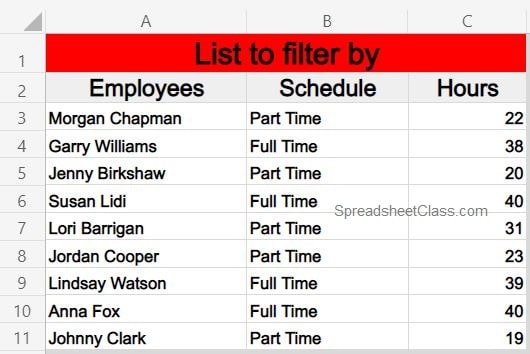
The list that you will use as the criteria in this example is on it's own tab, as shown above.

Directly below is the "Unfiltered Data". As you can see the COUNTIF function is being used like in the previous examples, to provide a clear indication of whether or not each row in the unfiltered data should appear in the filter results (Whether or not the name in column A is found in the "List to filter by").

List to filter by and formula on the same sheet

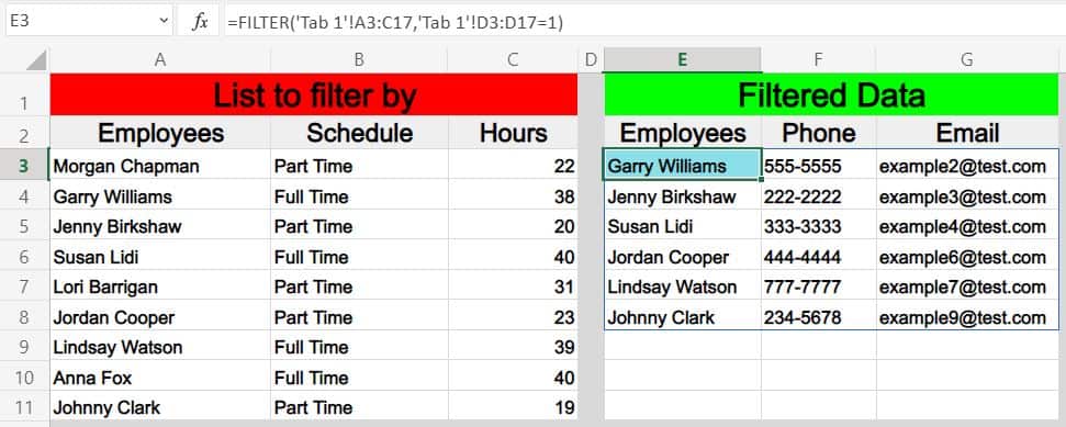
Here is an example showing how to set up your formula when the list that you want to filter by and the formula are on the same tab, but the unfiltered source data is on a separate tab.

Unfiltered source data & COUNTIF function: Tab 1

List to filter by: Tab 2

FILTER formula: Tab 2

The formulas: The COUNTIF formula below, is entered in cell D3 on Tab 1, and is copied into the cells below it to fill column D. The FILTER formula below is entered in cell E3 in Tab 2.

=COUNTIF('Tab 2'!A2:A12,A3)

=FILTER('Tab 1′!A3:C17,'Tab 1'!D3:D17=1)

Source data, list to filter by, and formula, all on separate sheets

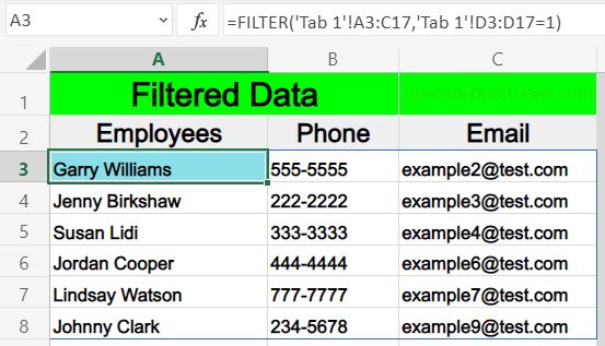
Finally, here is an example showing how to set up your formula when the unfiltered source data (data to be filtered), the list to filter by, and the formula are each on a separate tab.

Unfiltered source data / COUNTIF function: Tab 1

List to filter by: Tab 2

FILTER formula: Tab 3

The formulas: The COUNTIF formula below, is entered in cell D3 in Tab 1, and is copied into the cells below it to fill column D. The FILTER formula below is entered in cell H3 in Tab 3.

=COUNTIF('Tab 2'!A2:A12,A3)

=FILTER('Tab 1′!A3:C17,'Tab 1'!D3:D17=1)

Pop Quiz: Test your knowledge

Answer the questions below about filtering based on a list, to refine your knowledge! Scroll to the very bottom to find the answers to the quiz.

Question #1

Which of the following formulas has a criteria range of C3:C10?

1. =FILTER(A3:C10,D3:D10=1)
2. =FILTER(A3:C10,C3:C10=1)
3. =FILTER(C3:C10,D3:D10=1)

Question #2

Which of the following formulas has a source range of A3:G?

1. =FILTER(C3:C10,G3:G10=1)
2. =FILTER(A3:C10,A3:A10=1)
3. =FILTER(A3:G10,D3:D10=1)

Question #3

True or False: The COUNTIF function can be used to create a "Criteria column" for the FILTER function.

1. True
2. False

---

Answers to the questions above:

Question 1: 2

Question 2: 3

Question 3: 1