

When filtering data in Google Sheets you may sometimes need to filter by an entire list of values, rather than by just a single/few specified values.
You can use the FILTER and COUNTIF functions to filter based on a list in Google Sheets. You can also achieve the same task by using the FILTER and MATCH functions, but this formula combination is slower and much more resource-intensive than using the FILTER COUNTIF combination, especially when filtering multiple thousands of rows of data.
Here are formulas that you can use to filter by a list in Google Sheets:
FILTER COUNTIF
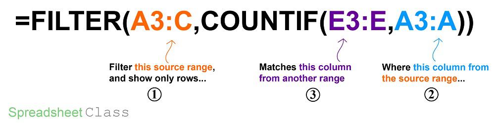
- =FILTER(A3:C,COUNTIF(E3:E,A3:A))
FILTER MATCH
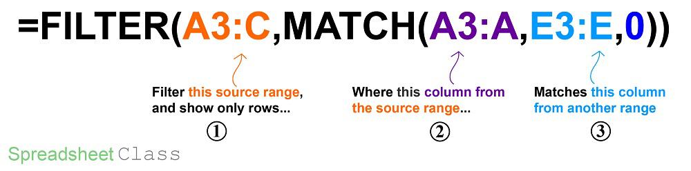
- =FILTER(A3:C,MATCH(A3:A,E3:E,0))
*Important Note: Do not confuse the formula(s) above with COUNTIF FILTER, which a completely different formula when nested/written in this order. COUNTIF FILTER is a formula which will count occurrences of a specified criteria within a filtered range, where FILTER COUNTIF will allow you to filter by a list of data.
This article focuses on filtering by a list in Google Sheets, but check out this article if you want to learn how to filter by a list in Excel.
Get the Google Sheets formulas cheat sheet
Overview:
In this article I will stick to using the FILTER and COUNTIF functions, since this is the faster and more reliable choice for filtering a range by an array in Google Sheets.
If you want to learn how to use the FILTER function to perform ordinary filtering tasks, here is an article that will help you learn the function from the ground up.
How to use the Google Sheets FILTER function
But here we will only be filtering by lists/arrays/columns of data.
How the formula works is fairly simple, but making sure that you have arranged your cell references in the right order can sometimes be confusing when filtering based on a list in Google Sheets, especially when filtering data from multiple tabs.
This is why I have provided multiple examples showing the different ways to set up the formula depending on how your data is arranged (i.e. depending on which tab your data/formula is on).
I have also provided the diagrams above to help you understand the formulas, how they work, and the type of data that each reference should point to.
Filter rows based on a list in another sheet
To start with, we will put our formula, our unfiltered data, and the list to filter by, all on the same tab so that you can easily see how the formula is set up and how it functions.
Filter a range by an array in Google Sheets
In this first example will start very simple, and filter a range of data, by a single-column / list, where the list that we are going to filter by does not contain any extra entries that are not present in the source data (data to be filtered).
This is not always how it will be in the real world… but this will make it easy to see what the formula is doing.
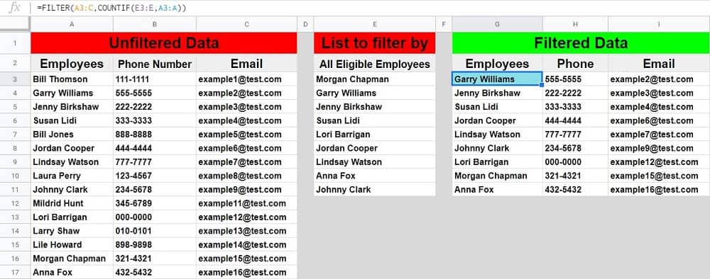
In this scenario, we have a set of data that shows a list of employees within an individual department at a company, as well as their contact information. We also have another list that shows employees within the department who are eligible for a bonus.
We are going to filter the data set that shows employees and their contact information, by the list of eligible employees… so that only the contact information data of eligible employees is displayed in the filter output.
Again, in this example, every employee that is on the “eligible” list will also be found within the unfiltered data.
The task: Show employee contact information for employees who are eligible for a bonus
The logic: Filter the range A3:C, where the values in the range A3:A are equal to any of the values in the range E3:E
The formula: The formula below, is entered in the blue cell (G3), for this example
=FILTER(A3:C,COUNTIF(E3:E,A3:A))
Filter a list by another list in Google Sheets
Now I am going to show you how to filter a list by another list in Google Sheets, or in other words how to filter a list by a single column.
This is similar to the last example, but here the employee contact information is not displayed, which can sometimes make it a little bit harder to determine what your source range is (range to be filtered).
When setting up your formula, always ask yourself, “which data is it that I am needing to filter?”, and then ask, “which data is it that I am needing to filter by?”.
Then refer to your formula diagram / cheat sheet to remember which range / reference goes where in the formula.
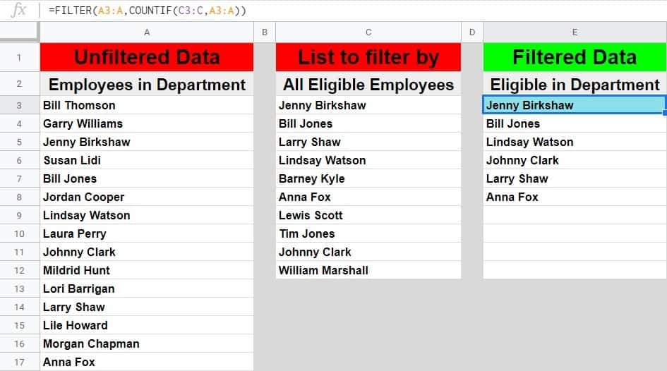
So once again, here we have a list of employees within an individual department at a company… but this time let’s say that the list of eligible (for a bonus) employees represents a company-wide list, and this means that only some of the employees on the eligibility list will be found within the source data/ list.
This will not affect how the formula operates but it’s good to note that your filter output will not show every single employee that is show on the eligibility list, as should be expected… since in this example only some employees are on both lists.
The task: Show a list of employees in your department, who are on the company-wide eligibility list
The logic: Filter the range A3:A, where the values in the range A3:A are equal to any of the values in the range C3:C
The formula: The formula below, is entered in the blue cell (E3), for this example
=FILTER(A3:A,COUNTIF(C3:C,A3:A))
Filter a range based on a column from another range
In this example, both the unfiltered source data (data to be filtered) and the list to filter by are given in the format of multiple column ranges. In other words, the list that we want to filter by is provided with other columns of data beside it this time.
This type of situation where the list to filter by is attached to other data can be expected in the real world… but it presents another potentially confusing situation with setting up your formula references because of the added columns.
This will not change how we setup the formula, and you may even notice that the formula in this example is the same formula that is used in the first example… but it is important to learn how to identify your column references with data that looks like this.
Again, if you are setting up a formula and you find yourself confused, just ask yourself which data needs to be filtered, and which data you are using to filter with/by, then refer to the diagram to find where each reference/range should be typed into the formula.
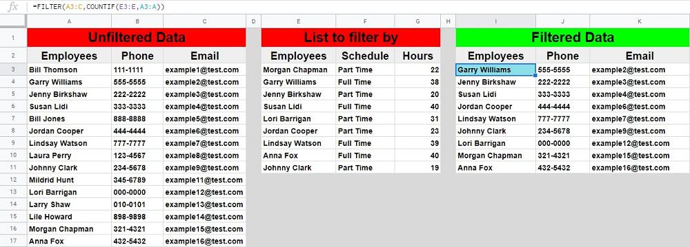
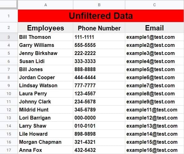
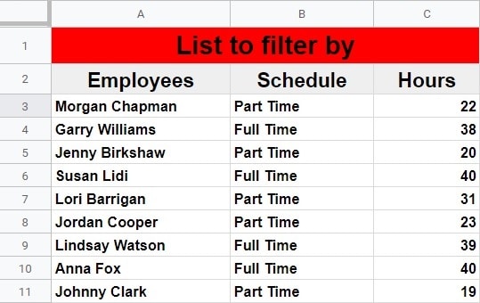
So in this scenario, let’s say that we have two different data reports that show employee information. One report shows employee contact information like in the previous examples, and the other report shows employee work schedules.
What we want to do is filter the contact information, by the list of employees who appear on the work schedule report. Pretend that your boss gave you these two different reports / sets of data, and said that he or she needed you to filter the contact information so that only the employees who are on the schedule are shown.
The task: Show employee contact information for the employees who appear on the work schedule
The logic: Filter the range A3:C, where the values in range A3:A are equal to any of the values in the range E3:E
The formula: The formula below, is entered in the blue cell (I3), for this example
=FILTER(A3:C,COUNTIF(E3:E,A3:A))
Filtering by a list when the data is on separate sheets
Now that you know how to filter by a list where all of the data and the formula are held on the same sheet/tab, let’s go over how to filter by a list when using multiple tabs.
There are a variety of arrangements that are possible when using multiple tabs for filtering a range by an array, and so I’ll go over each of them.
We will use the same exact data and task as in the last example, to make things simple and to allow for easy comparison.
Source data and formula on the same sheet
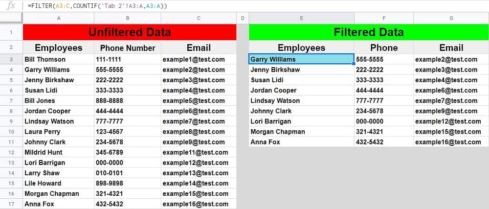
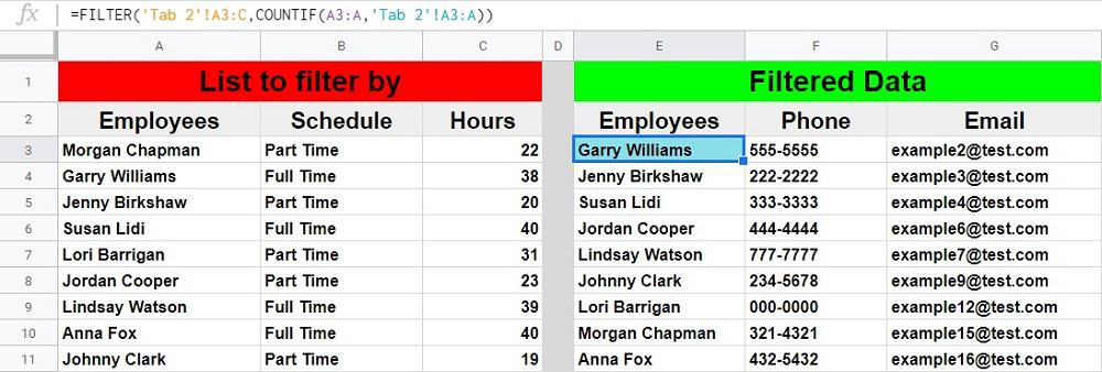
Here is an example showing how to set up your formula when the unfiltered source data and filter formula are on the same tab… but where your list that you want to filter by is on a separate tab.
Unfiltered source data: Tab 1
Formula: Tab 1
List to filter by: Tab 2
The formula: The formula below, is entered in the blue cell (E3), for this example
=FILTER(A3:C,COUNTIF(‘Tab 2’!A3:A,A3:A))

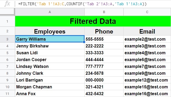
List to filter by and formula on the same sheet
Here is an example showing how to set up your formula when the list that you want to filter by and the formula are on the same tab, but the unfiltered source data is on a separate tab.
List to filter by: Tab 1
Formula: Tab 1
Unfiltered source data: Tab 2
The formula: The formula below, is entered in the blue cell (E3), for this example
=FILTER(‘Tab 2′!A3:C,COUNTIF(A3:A,’Tab 2’!A3:A))
Source data, list to filter by, and formula, all on separate sheets
Finally, here is an example showing how to set up your formula when the unfiltered source data (data to be filtered), the list to filter by, and the formula are each on a separate tab.
Unfiltered source data: Tab 1
List to filter by: Tab 2
Formula: Tab 3
The formula: The formula below, is entered in the blue cell (A3), for this example
=FILTER(‘Tab 1’!A3:C,COUNTIF(‘Tab 2′!A3:A,’Tab 1’!A3:A))

FILTER COUNTIF diagram: (Recommended formula)
FILTER MATCH diagram: (Recommended to use FILTER COUNTIF instead)
You’ll notice that even though the FILTER COUNTIF and FILTER MATCH formulas look very similar and perform the exact same task, the references used in these formulas are in a different order.
How I filter based on a list at my job
In my work, the way that I use the formulas on this page is to filter students data, given a list of student IDs.
For example if someone sends me a list of students to investigate, I take the list of their ID numbers, and filter by that list to retrieve the data (such as attendance) for only the students in the list.
Pop Quiz: Test your knowledge
Answer the questions below about filtering based on a list, to refine your knowledge! Scroll to the very bottom to find the answers to the quiz.
Classroom downloads:
Filter by list cheat sheet (PDF)
Google Sheets formulas cheat sheet
Click the green “Print” button below to print this entire article.
Question #1
Which of the following formulas filters a range, by the column/range C3:C?
- =FILTER(A3:G,COUNTIF(Z3:Z,A3:A))
- =FILTER(B3:C,COUNTIF(A3:A,B3:B))
- =FILTER(D3:J,COUNTIF(C3:C,E3:E))
Question #2
Which of the following formulas has a source range of A3:G?
- =FILTER(A3:G,COUNTIF(Z3:Z,A3:A))
- =FILTER(B3:C,COUNTIF(A3:A,B3:B))
- =FILTER(D3:J,COUNTIF(C3:C,E3:E))
Question #3
True or False: FILTER COUNTIF and FILTER MATCH do the same thing?
- True
- False
Answers to the questions above:
Question 1: 3
Question 2: 1
Question 3: 1