

The FILTER function is a very useful and frequently used function, that you will likely find the need for in many situations. The Google Sheets FILTER function allows you to filter your data based on any criteria that you want, automatically with a formula.
In this lesson I will show you several different ways to use the FILTER formula in Google Sheets, including how to filter by multiple conditions / criteria.
To filter by using the FILTER function in Google Sheets, follow these steps:
- Type =FILTER( to begin your filter formula
- Type the address for the range of cells that contains the data that you want to filter, such as A1:B
- Type a comma, and then type the condition for the filter, such as B1:B>3 (To set a condition, first type the address of the “criteria column” such as B1:B, then type an operator such as greater than (>), and then type the criteria, such as the number 3.
- Type a closing parenthesis and then press enter on the keyboard. Your entire formula will look like this: =FILTER(A1:B,B1:B>3)
In this article I will start with the basics of using the FILTER function (examples included), and then also show you some more advanced ways of using the FILTER function. This article focuses specifically on the FILTER function that is typed into the spreadsheet cells as a formula, and not the filter command available from the toolbar and pop-up menus.
Using the FILTER function in Google Sheets is almost the same as using it in Excel, but there are slight differences between the two. Click here to read the Excel version of this article
Click here to get your Google Sheets cheat sheet
The Google Sheets FILTER function:
The diagram below will show you exactly how the FILTER function works in Google Sheets.
=FILTER(A3:B, B3:B=F1)
(Copy/Paste the formula above into your sheet and modify as needed)
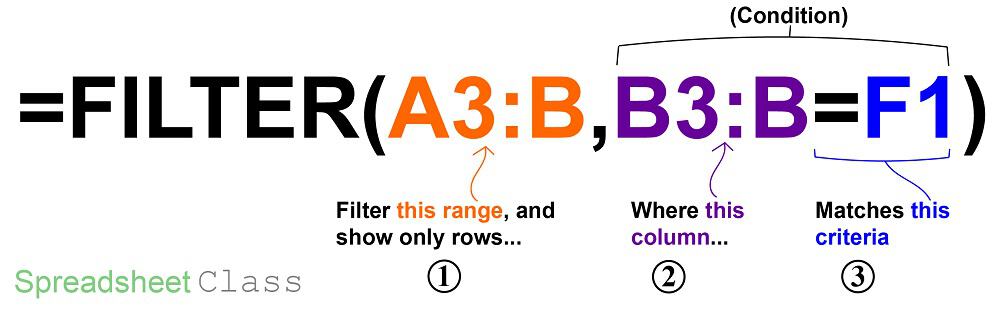
The FILTER function in Google Sheets allows you to filter a range of data by a specified condition, so that a new set of data will be displayed which only shows the rows/columns from the original data set that meets the criteria/condition set in the formula.
Here are the types of Filter formulas that I will teach you:
Here are the formulas that we will cover in this lesson. Further below are detailed examples with images included.
- Filter by a number
- Filter by a cell value
- Filter by a text string
- Filter where NOT equal to
- Filter by date
- Filter to find largest / smallest values
- Filter by multiple conditions
- Filter from another sheet
Google Sheets description for FILTER function:
Syntax:
FILTER(range, condition1, [condition2, …])Formula summary: “Returns a filtered version of the source range, returning only rows or columns which meet the specified conditions.”
The source range that you want to filter, can be a single column or multiple columns.
The range that is used to check against the criteria that you set, must be a single column (later I will show you how to filter by multiple conditions, but don’t worry about that for now).
The criteria that is set in the condition can be manually typed into the formula as a number or text, or it can also be a cell reference.
*Note that the source range and the single column range for the condition must be the same size (must contain the same number of rows), or the cell will display an error that says “filter has mismatched range sizes“.
This article focuses on filtering vertically, which is the most common way of using the FILTER function in Google Sheets. But if you want to learn how to filter horizontally, check out the article that is linked below.
How to filter horizontally in Google Sheets
Filtering by a single condition in Google Sheets
First let’s go over using the FILTER function in Google Sheets in its simplest form, with a single condition/criteria.
I will show you how to filter by a number, a cell value, a text string, a date… and I will also show you how to use varying “operators” (Less than, Equal to, etc…) in the filter condition.
How to filter by a number
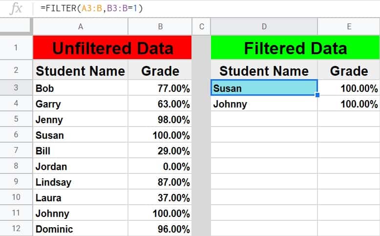
In this first example on how to use the filter function in Google Sheets, the scenario is that we have a list of students and their grades, and that we want to make a filtered list of only students who have a perfect grade.
The task: Show a list of students and their scores, but only those that have a perfect grade
The logic: Filter the range A3:B, where the column B3:B is equal to 1 (100%)
The formula: The formula below, is entered in the blue cell (D3), for this example
=FILTER(A3:B, B3:B=1)
Operators that can be used in the FILTER function:
In this example we are using the operator “=” (Equal To) for the filter condition/criteria, but you can also use any of the following:
“=” (Equals)
“>” (Greater than)
“<” (Less than)
“<>” (Not equal to)
“>=” (Greater than or equal to)
“<=” (Less than or equal to)
How to filter by a cell value in Google Sheets
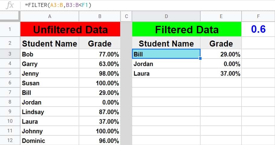
In this example, we want to achieve the same goal as discussed above, but rather than typing the condition that we want to filter by directly into the formula, we are using a cell reference.
When you filter by a cell value in Google Sheets, your sheet will be set up so that you can change the value in the cell at any time, which will automatically update the value that the filter criteria it attached to.
In this example, you will notice that instead of directly typing the number “0.6” into the formula itself, the filter criteria is set as cell G1, where the “0.6” value is entered.
The task: Show a list of students and their scores, but only those that have a failing score
The logic: Filter the range A3:B, where B3:B is less than the value that is entered in the cell F1 (0.6)
The formula: The formula below, is entered in the blue cell (D3), for this example
=FILTER(A3:B, B3:B<F1)
How to filter by text
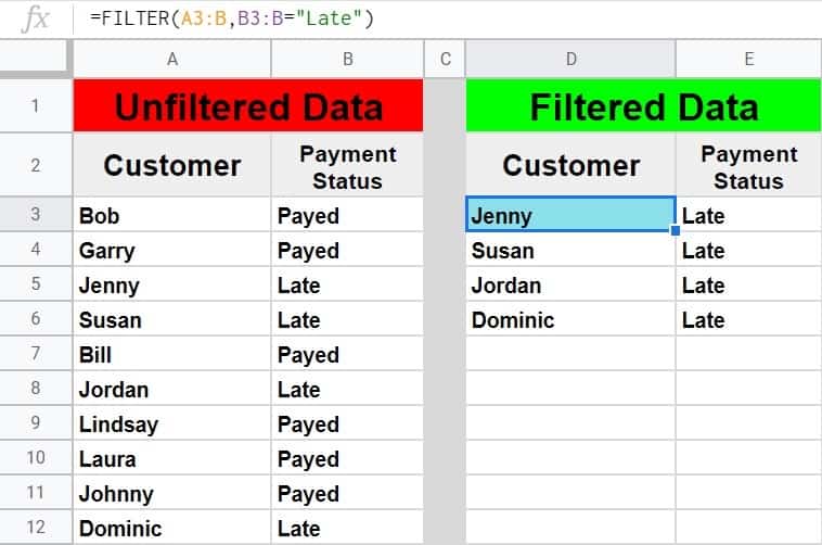
In this example, we are going to use a text string as the criteria for the filter formula. This is very similar to using a number, except that you must put the text that you want to filter by inside of quotation marks.
In this scenario we are filtering a list that shows customers and their payment status, and we want to display only customers that have a payment status of “Late”.
The task: Show a list of customers who are past due on their payments
The logic: Filter the range A3:B, where B3:B equals the text, “Late”
The formula: The formula below, is entered in the blue cell (D3), for this example
=FILTER(A3:B, B3:B=”Late”)
Using NOT EQUAL TO in the Google Sheets FILTER function
Now that you have got a basic understanding of how to use the filter function in Google Sheets, here is another example of filtering by a string of text, but in this example we will use the “not equal” operator (<>), so that you can learn how to filter a range and output data that is NOT equal to criteria that you specify.
In this example we will also use a larger data set to demonstrate a more extensive application of the FILTER function in the real world.
You may be surprised at how often a situation comes up when you need to filter data where it is “not equal to” a certain number or piece of text that you specify.
In this example let’s say that we have a report/spreadsheet that shows data from sales calls that occur at your company, and we want to filter the data so that a specified sales rep (Bob) is NOT included in the filter output.
The task: Show sales call data for all sales reps, except Bob
The logic: Filter the range A2:E, where B2:B DOES NOT equal the text, “Bob”
The formula: The formula below, is entered in the blue cell (G3), for this example
=FILTER(A3:E, B3:B<>”Bob”)
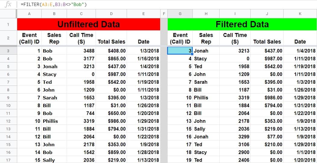
Notice that the filtered data on the right side of the image above does not contain any of the rows/calls that Bob was involved in.
How to filter by date in Google Sheets
Filtering by a date in Google Sheets can be done in a couple of ways, which I will show you below. If you try to type a date into the FILTER function like you normally would type into a cell… the formula will not work correctly.
So you can either type the date that you want to filter by into a cell, and then use that cell as a reference in your formula… or you can use the DATE function.
When filtering by date you can use the same operators (>, <, =, etc…) as in other FILTER function applications. In Google Sheets each different day/date is simply a number that is put into a special visual format.
For example, in Google Sheets, the date “06/01/2019” is simply the number “43,617”, but displayed in date format. When you add one day to the date, this number increments by one each time… i.e “43,618” “43,619” “43,620”
So, one date can be considered to be “greater than” another date, if it is further in the future. Conversely, one date can be said to be “less than” another date, if it is further in the past.
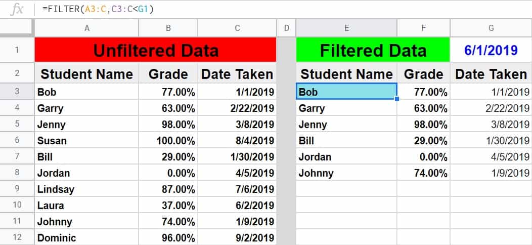
In this first example we will filter by a date by using a cell reference. This is similar to the example we went over in part 2, but in this example instead of working with percentages, we are dealing with dates.
Let’s say that we want to filter a list of students, their test scores, and the dates that the tests were completed… and we want to show only tests that were taken before June (06/01/2019).
Filter by date in Google Sheets example 1:
The task: Show only tests that were taken before June
The logic: Filter the range A3:C, where C3:C is less than the date that is entered in cell G1 (06/01/2019)
The formula: The formula below, is entered in the blue cell (E3), for this example
=FILTER(A3:C,C3:C<G1)
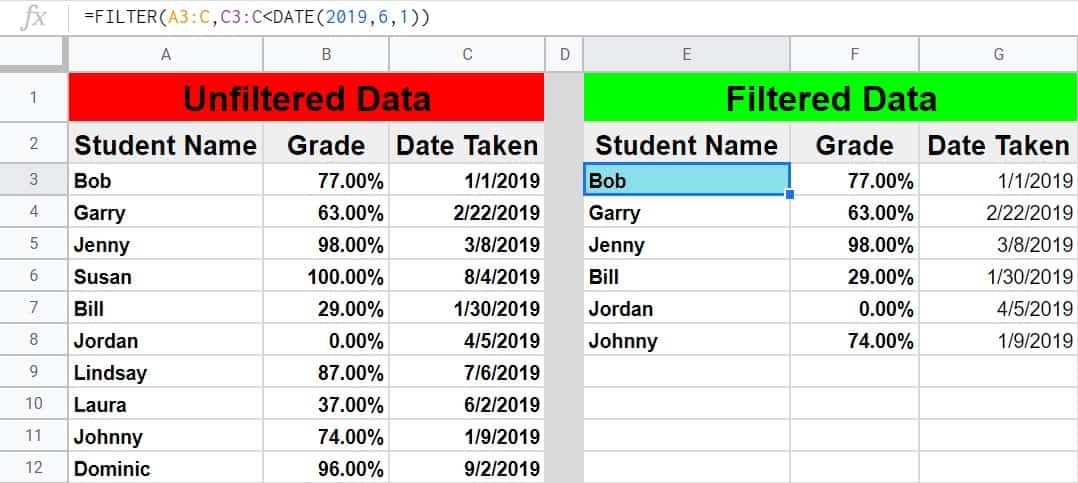
Filter by date in Google Sheets example 2:
In this second example on filtering by date in Google Sheets we are using the same data as above, and trying to achieve the same results… but instead of using a cell reference, we will use the DATE function so that you can type enter the date directly into the FILTER function.
When using the DATE function to designate a certain date, you must first enter the year, then the month, and then the day… each separated by commas (shown below).
The task: Show only tests that were taken before June
The logic: Filter the range A3:C, where C3:C is less than the date of (06/01/2019)
The formula: The formula below, is entered in the blue cell (E3), for this example
=FILTER(A3:C,C3:C<DATE(2019,6,1))
Filter to display the largest or smallest values
You can also filter data to display only the largest or smallest values. I will teach you multiple ways to do this.
Filter to display the largest values (Top 10, Top 100, etc.)
We can filter to display only the largest values by using the FILTER function with the LARGE function. This will allow you to specify how many results you want to display, such as the top 3, top 10, top 100, etc.
=Filter(A3:B,(B3:B>=LARGE(B3:B,3)))
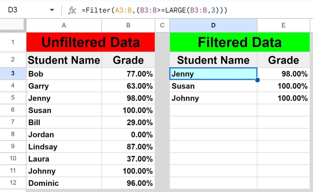
As you can see in the image above, the student names & student scores are being filtered to display only the students with the 3 highest scores. Simply change the number “3” in the LARGE function to any number that you want, to specify how many rows / how many results you want to display.
The formula below uses the SORT function in combination with the formula above, to display the largest results in descending order (largest first):
=Sort(Filter(A3:B,(B3:B>=LARGE(B3:B,3))),2,false)
Alternative method:
Although this method does not actually use the FILTER function, it still does the same thing as the formula in the example above. This method is my preference.
You can use the SORT function with the ARRAY_CONSTRAIN function to display the largest values. This simply sorts the data in descending order, and then displays the specified number of results from the top.
The formula below is an example of how to use this method.
=ARRAY_CONSTRAIN(SORT(A3:B,2,false),3,2)
Filter to display the smallest values (Bottom 10, Bottom 100, etc.)
We can filter to display only the smallest values by using the FILTER function with the SMALL function. This will allow you to specify how many results you want to display, such as the bottom 3, bottom 10, bottom 100, etc.
=Filter(A3:B,(B3:B<=SMALL(B3:B,3)))
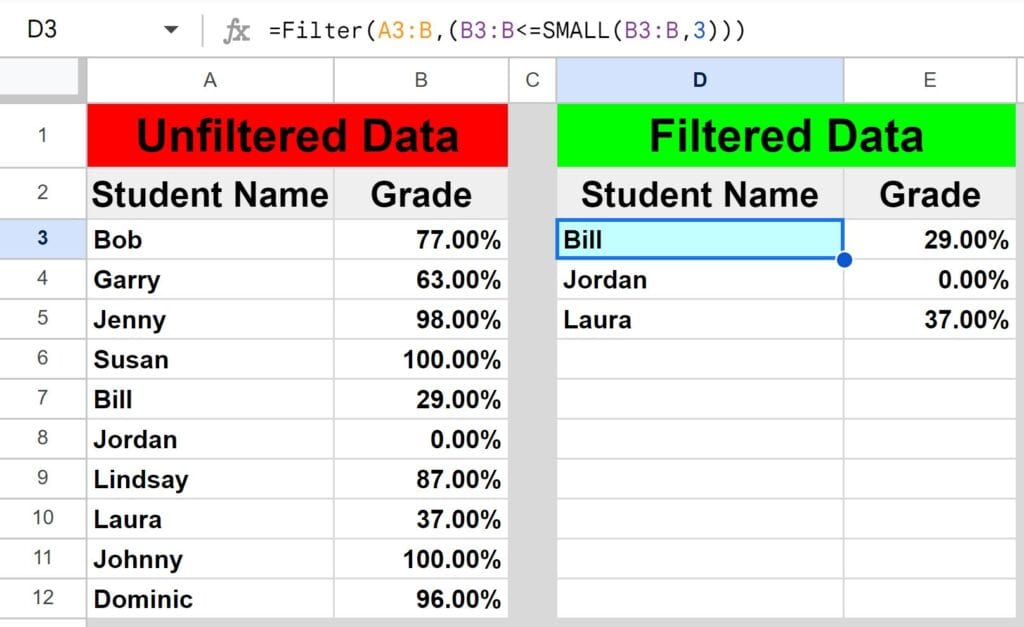
As you can see in the image above, the student names & student scores are being filtered to display only the students with the 3 lowest scores. Simply change the number “3” in the SMALL function to any number that you want, to specify how many rows / how many results you want to display.
The formula below uses the SORT function in combination with the formula above, to display the smallest results in ascending order (smallest first):
=sort(Filter(A3:B,(B3:B<=SMALL(B3:B,3))),2,true)
Alternative method:
The same method from the previous example can be used to find the smallest values, by using the SORT function with the ARRAY_CONSTRAIN function to display the largest values. Except in this case, the formula sorts the data in ascending order, and then displays the specified number of results from the top.
The formula below is an example of how to use this method.
=ARRAY_CONSTRAIN(SORT(A3:B,2,true),3,2)
Filter by multiple conditions in Google Sheets
When using the Google Sheets FILTER function you may want to output a set of data that meets more than just one criteria. I will show you two ways to filter by multiple conditions in Google Sheets, depending on the situation that you are in, and depending on how you want the formula to operate.
The normal way of adding another condition to your filter function, (as shown by the formula syntax in Google Sheets), will allow you to set a second condition, where the first AND second condition must be met to be returned in filter output.
However I will also show you how to make a slight modification to the function so that you can choose to set a second condition where EITHER condition can be met to return/display in the filter function’s output/destination. (Separate the conditions with a comma to use AND logic, or separate the conditions with a plus sign to use AND logic.)
If you want to learn how to filter based on an entire list/column, check out the article below.
“How to filter based on a list in Google Sheets”
Filtering by 2 conditions where BOTH MUST BE TRUE
In this example, we are going to filter a set of data, and only display rows where BOTH the first condition AND the second condition are met/true.
To use a second condition in this way (with AND logic), simply enter the second condition into the formula after the first condition, separated by a comma (shown below).
When using the filter formula with multiple conditions like this, the columns that are referenced in each condition must be different.
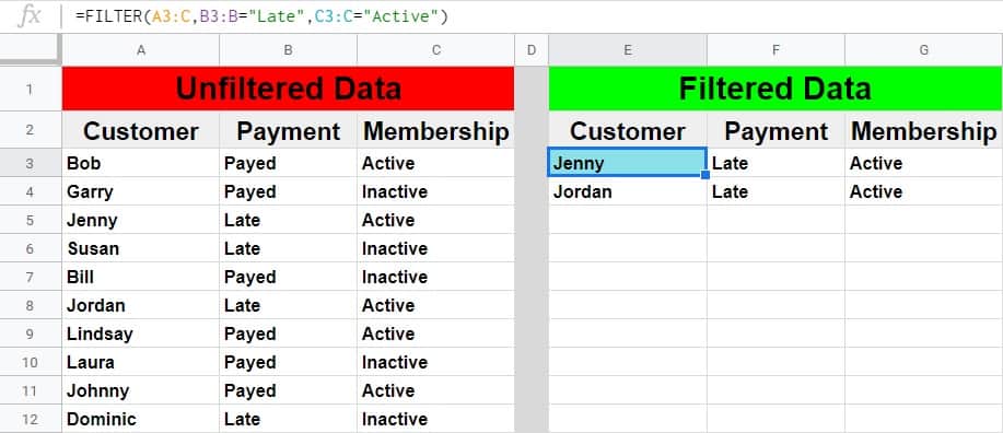
In this scenario we want to filter a list that shows customers, their payment status, and their membership status… and to show only customers who have an active membership AND who are also late on their payment.
This will make sure that customers with an inactive membership who are still designated as being late on payment in the system… are not shown in the filter results, and not put on the list for being sent a “late payment” notice.
The task: Show a list of customers who are late on their payments, but only those with active memberships
The logic: Filter the range A3:C, where B3:B equals the text “Late”, AND where C3:C equals the text “Active”
The formula: The formula below, is entered in the blue cell (E3), for this example
=FILTER(A3:C, B3:B=”Late”, C3:C=”Active”)
Filtering by 2 conditions where EITHER ARE TRUE, not necessarily both
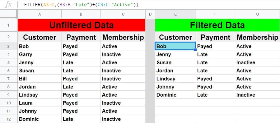
In this example we are going to filter a set of data and only display rows where EITHER the first condition OR the second condition are met/true.
To use a second condition in this way (with OR logic), simply enter the second condition into the formula after the first condition, separated by a plus sign. Each condition must be inside of its own set of parenthesis (shown below).
When using the FILTER formula in this way, you can choose criteria from the same or different columns.
In this scenario we want to filter the same customer data as shown in the previous example, but this time we want to show a list of customers who EITHER have an active membership OR who are late on their payment.
This will give a list of customers who can be sent a notice for payment… including active members, or/also inactive members who are late on their final payment.
The task: Show a list of customers who are active members, and include customers who are late on payment even if they are not active members
The logic: Filter the range A3:C, where B3:B equals the text “Late”, OR where C3:C equals the text “Active”
The formula: The formula below, is entered in the blue cell (E3), for this example
=FILTER(A3:C, (B3:B=”Late”)+(C3:C=”Active”))
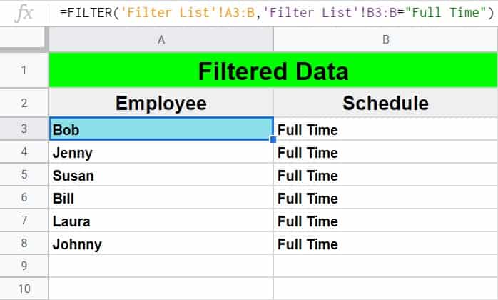
How to filter from another sheet in Google Sheets
You may often find situations where you need to filter from another sheet in Google Sheets, where your raw unfiltered data is on one tab, and your filter formula / filter output is on another tab.
This can be done by simply referring to a certain tab name when specifying the ranges in the filter. So where you would normally set a range like “A3:B”, when referencing another sheet while filtering you specify the tab name by adding the tab name and an exclamation mark before the column/row portion of the range, like “TabName!A3:B”
However when the tab name has a space in it, it is necessary to use an apostrophe before and after the tab name, like ‘Tab Name’!A3:B.
Here is an example of how to filter data from another tab in Google Sheets, where your filter formula will be on a different tab than the source range.
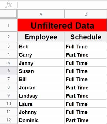
Let’s say that you have a list of employees and their schedule type (Full Time / Part Time) on one tab, and that you want to display a filtered list of full time employees on another tab.
The task: Filter the list of employees on the tab labeled “Filter List”, and show a list of employees who have a full time schedule, on a separate tab
The logic: Filter the range ‘Filter List’!A3:B, where the range ‘Filter List’!B3:B is equal to the text “Full Time”
The formula: The formula below, is entered in the blue cell (A3), for this example
=FILTER(‘Filter List’!A3:B,’Filter List’!B3:B=”Full Time”)
Here is a list of employees and their schedules, which is held on a tab labeled “Filter List”
And here is a filtered list of employees who have full time schedules, where the filter formula and output data are held on a separate tab
Using the FILTER function with the SORT function
In Google Sheets you can combine multiple functions into a single formula, so that the formula performs the task of two functions all at once.
In the video below (or the article linked below), I will show you how to use the FILTER function with the SORT function, as individual functions, and in a single formula!
But as a quick example, here is what a formula looks like, that both sorts and filters (contains both the SORT and FILTER function).
=SORT(FILTER(A3:C,C3:C=”Text”),1,true)
The formula above filters columns A through C, where column C is equal to “Text”, and then the formula sorts the filter results by the first column in ascending order.
Learn how to use the SORT function with the FILTER function.
When no matches are found
When no matches are found, Google Sheets will display an error message that looks like the image below. The cell will say “#N/A” and when you hover your cursor over the cell a message will pop up that says “No matches are found in FILTER evaluation“.
This simply means that there are no results from the source data that matches your criteria.
This is not always an actual error. For example, if you are filtering to display students with a score of 100%, and there are no students with a grade of 100%, then no matches will be found and the error message will pop up. In this case, the formula is correct but there are simply no results.
Sometimes this message will display when you have entered the wrong criteria in your function. For example, let’s say that you meant to filter to only display students who have a grade that is above 70%, but you forget to put a decimal point in your criteria and use the number “7” instead of “0.7”. This would cause an error since 7 = 700% and no student can have a score above 100%.
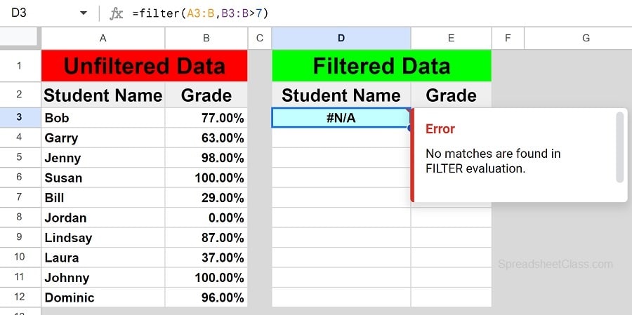
So when you encounter this error, simply look at your criteria and make sure that it is correct. If it is correct, then that means there are simply no matches from the source data that meet the criteria given.
Filter where the criteria is contained in the cell
If you want, you can filter your data to display only the rows that contain the specified criteria, instead of the criteria needing to be an exact match.
For example, let’s say that you want to filter your data to display only the rows where cells in column A contain the word “Task”. You want the cells that say “Task 1” and “Task 2” etc. to display in your filter results, because they contain the word “Task”, even though they are not an exact match.
This is a more advanced lesson that I have covered in detail here in this article on filtering where the cells contain the given criteria.
Let’s review the Google Sheets Filter formulas:
Here are the formulas that we covered in this lesson.
Filter by a number
- =FILTER(A3:B, B3:B=1)
Filter by a cell value
- =FILTER(A3:B, B3:B<F1)
Filter by a text string
- =FILTER(A3:B, B3:B=”Late”)
Filter where NOT equal to
- =FILTER(A3:E, B3:B<>”Bob”)
Filter by date
- =FILTER(A3:C,C3:C<G1) (Date entered in cell G1)
- =FILTER(A3:C,C3:C<DATE(2019,6,1))
Filter by multiple conditions
- =FILTER(A3:C, B3:B=”Late”, C3:C=”Active”) (AND logic)
- =FILTER(A3:C, (B3:B=”Late”)+(C3:C=”Active”)) (OR logic)
Filter from another sheet
- =FILTER(‘Sheet Name’!A3:B,’Sheet Name’!B3:B=”Full Time”)
How I use the FILTER formula in my work
This particular formula is incredibly useful and the list of ways that I use it at my job go on and on.
But in general I use it to do 1 main thing. Creating lists of students that meet specified criteria. Students who are “active”, students how have failing grades, students who have not completed their assessment, etc.
It’s an essential formula for creating focus lists. If you nail down the right filter criteria in your data, you can I identify the products or services or employees or students that are performing the best, the worst, etc.
Pop Quiz: Test your knowledge
Answer the questions below about the Google Sheets FILTER function, to refine your knowledge! Scroll to the very bottom to find the answers to the quiz.
Classroom downloads:
FILTER function cheat sheet (PDF)
Click here to get your Google Sheets cheat sheet
Or click here to take the dashboards course
Click the green “Print” button below to print this entire article.
Question #1
Which of the following formulas uses a “cell reference” in the filter condition?
- =FILTER(A1:D, B1:B<0.6)
- =FILTER(A2:C, C2:C=F1)
- =FILTER(A:P, G:G=”Yes”)
Question #2
Which of the following formulas uses the “Not Equal” operator?
- =FILTER(C:T, J:J>100)
- =FILTER(A:B, B:B=”No”)
- =FILTER(S:Z, T:T<>”True”)
Question #3
True or False: If the column(s) in the source range and the column in the filter condition are not the same size (if one has more rows than the other), the formula will not work, and will display an error.
- True
- False
Question #4
Which of the following formulas uses AND logic, where BOTH conditions must be met to satisfy the filter criteria?
- =FILTER(C:F, (F:F=”Yes”)+(E:E=”Active”))
- =FILTER(C:F, F:F=”Yes”, E:E=”Active”)
Question #5
Which of the following formulas uses OR logic, where EITHER condition can be met to satisfy the filter criteria?
- =FILTER(A:K, K:K=”Yes”, J:J=”Active”)
- =FILTER(A:K, (K:K=”Yes”)+(J:J=”Active”))
Answers to the questions above:
Question 1: 2
Question 2: 3
Question 3: 1
Question 4: 2
Question 5: 2