

When you are filtering data in Google Sheets with the FILTER function, in most cases you will probably use it to filter vertically, however you may sometimes have data that needs to be filtered horizontally. With a slight adjustment to your references in the filter formula, you can filter horizontally, where you are filtering columns instead of rows.
To filter horizontally in Google Sheets, do the following:
- Enter the source range into your FILTER function, for example A1:2. This range represents the columns that you want to filter
- Set the criteria range in the filter condition, for example A2:2. This range represents the row that you will check your criteria against
- Set the criteria, for example =50. This criteria designates the values that must be contained in the criteria row in order to have a column display in the filter output
- After following the steps above, your horizontal filter formula will look like this =FILTER(A1:2,A2:2=50)
In comparison to using the Google Sheets FILTER function vertically, notice that in the instructions above, the source range refers to columns instead of rows, and the criteria range refers to a row instead of a column.
Get your Google Sheets formula cheat sheet
Horizontal FILTER formula
The diagram below shows how a horizontal FILTER formula is setup, and describes what each part of the formula does.
Horizontal filter formula example: =FILTER(C1:2,C2:2>100)
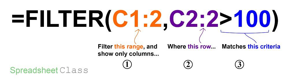
When setting up you FILTER function so that it will filter horizontally, your source range can be a single row or multiple rows if you want it to be, but your criteria range (the range that contains the values to check against) must be a single row… in the same way that when filtering normally/vertically, the criteria range must be a single column.
Also note that when filtering horizontally, your source range and your criteria range must contain the same number of columns (i.e. must start and end on the same column), or you will see an error appear that says “Filter has mismatched range sizes“.
With the FILTER function you can use numbers, text, or even cell references as the criteria for your formula:
- When using a number for the filter criteria, it will look something like <10
- When using text for the filter criteria, you must include quotation marks before and after the text, like this =”Text”
- When using a cell reference as your filter criteria, it will look something like this >K3
So let’s go over a few examples of how to use the FILTER function to horizontally filter sets of data in Google Sheets.
In the examples below, I’ll show you how to filter (horizontally) by numbers, by strings of text, and by cell references too!
How to filter horizontally in Google Sheets
First, let’s start with a simple example, where we will filter a small set of data horizontally, by a number.
Let’s say that you have data showing the total number of visitors per day at an event that you are running, and that you want to see which days lots of people attended on.
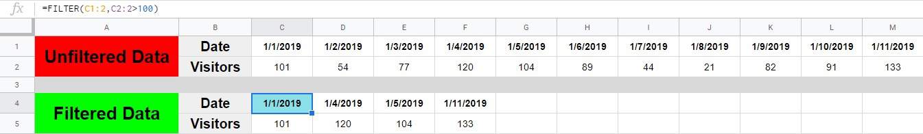
In rows 1 and 2 in the example shown below, the total number of visitors per day are listed horizontally over an eleven day period.
We are going to filter this data, so that we can see the days that had more than 100 visitors.
The task: Filter the data showing total visitors per day, to display only days with a high number of visitors
The logic: Filter the range C1:2, and display only columns where the range C2:2 is greater than 100
The formula: The formula below, is entered in the blue cell (C4), for this example
=FILTER(C1:2,C2:2>100)
Filtering average assignment grades
When listing assignment grades in a class, it is common to list the assignments horizontally across the top of the sheet, with the students listed vertically down the left side of the sheet.
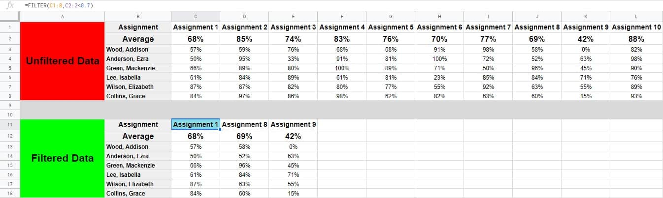
In this example we will filter a set of data that shows the assignment grades (scores) for several students and the average assignment grade in the class, based on the individual student scores.
With the data setup in this way, to filter by average assignment grade, you will need to filter horizontally.
Let’s say that you want to see only the assignments that have an average grade of over 70%, listed along with the individual student scores for those same assignments.
The task: Filter the assignment scores, and show only the assignments that have a combined average of more than 70% percent
The logic: Filter the range C1:8, and display only the columns where the range C2:2 is greater than 0.7
The formula: The formula below, is entered in the blue cell (C11), for this example
=FILTER(C1:8,C2:2<0.7)
How to filter horizontally by text
Now let’s go over an example where a string of text is the criteria that you want to filter by.
Remember that when using text as the criteria for your filter, you must use quotation marks before and after the text.
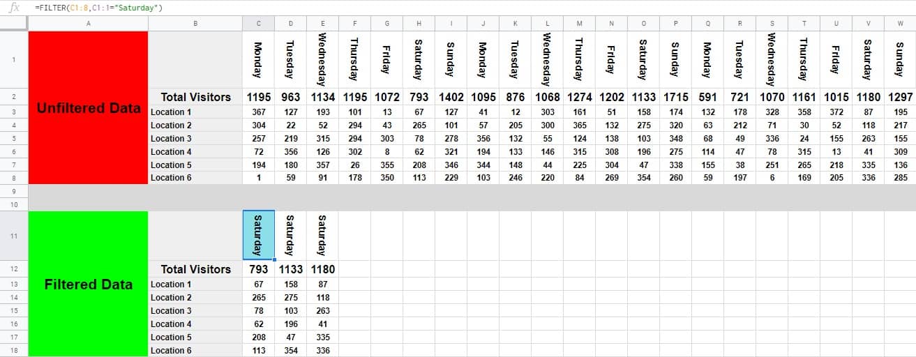
In this example we have a set of data that shows the number of visitors for multiple store locations on each day, as well as the total number of visitors on each day with all stores combined.
Let’s say that you need to see the totals for Saturdays only. You can isolate the data that pertains to Saturdays by using the FILTER function to filter the data shown below, horizontally.
The task: Show the total number of visitors, for Saturdays only
The logic: Filter the range C1:8, and display only the columns where the range/row C1:1 equals the text “Saturday”
The formula: The formula below, is entered in the blue cell (C11), for this example
=FILTER(C1:8,C1:1=”Saturday”)
How to filter horizontally by a cell reference
Finally, let’s go over how to use a cell reference as your filter criteria in your horizontal filter formula.
When you use a cell reference as your criteria, the value that is entered into the referenced cell, is the value that the filter formula will use to check data against. In other words, the value in the cell, is the value that your filter formula will use as the criteria.
An advantage of referring to a cell for specifying your filter criteria, is that it makes it very easy to adjust the criteria without having to modify the formula.
In this example we will use the same set of data from the previous example, but we will achieve a different task, with a different set of criteria.
Let’s say that you want to filter the data that shows visitors per day, to see which days had the greatest number of total visitors, and to determine whether certain days of the week have a tendency to attract lots of people.
To do this, we will create a filter formula that only shows us the days that had more than 1200 total visitors.
This is very similar to the first example, except that in this case, instead of typing the number directly into the formula… we will type the number that we are filtering by into a spreadsheet cell, and then refer to that cell in the filter condition.
The task: Show only data from the days that had more than 1200 total visitors
The logic: Filter the range C1:8, and display only the columns where the range C2:2 is equal to the value that is in cell B10 (1200).
The formula: The formula below, is entered in the blue cell (C10), for this example
=FILTER(C1:8,C2:2>B10)
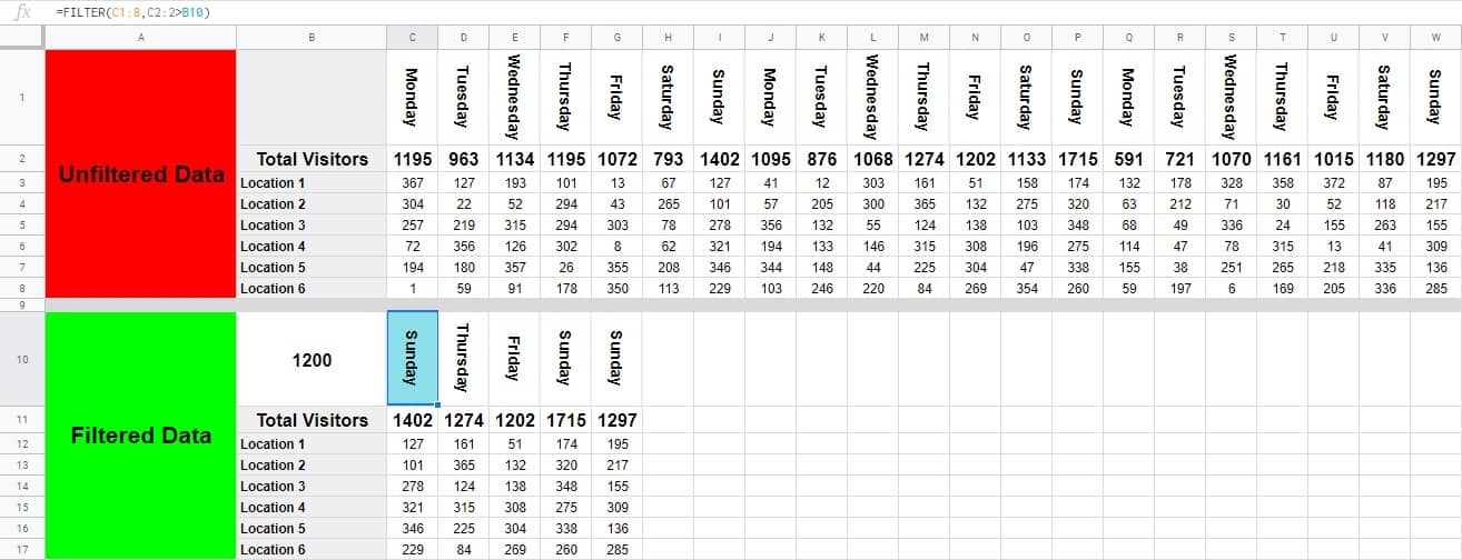
As you can see in the example below, the filtered data suggests that Sunday tends to be a busy day.
Pop Quiz: Test your knowledge
Answer the questions below on filtering horizontally, to refine your knowledge! Scroll to the very bottom to find the answers to the quiz.
Classroom downloads:
Horizontal FILTER cheat sheet (PDF)
Get your Google Sheets formulas cheat sheet
Click the green “Print” button below to print this entire article.
Question #1
Which of the following formulas will filter horizontally?
- =FILTER(A:B,A:A>6)
- =FILTER(D10:15,D11:11=9)
- =FILTER(D10:G,E10:E=1)
Question #2
Which of the formulas below uses row 3 as a criteria row?
- =FILTER(G1:Z3,G8:Z8=0)
- =FILTER(C3:9,C9:9=”Yes”)
- =FILTER(A3:9,A3:3=”No”)
Question #3
True or False: This formula is a valid horizontal filter formula =FILTER(1:3,1:1=1)
- True
- False
Question #4
Which of the following formulas uses rows 3 through 7 for its source range?
- =FILTER(Z3:7,Z6:6>100)
- =FILTER(A1:G7,A3:G3<1000)
Question #5
Which of the following formulas will not function properly because of a mismatched range size?
- =FILTER(A2:100,A33:33<777)
- =FILTER(J1:2,K2:2=10)
Answers to the questions above:
Question 1: 2
Question 2: 3
Question 3: 1
Question 4: 1
Question 5: 2