

If you want to filter your data and transpose it with a single formula in Google Sheets, you can do this by combining the FILTER function with the TRANSPOSE function. The FILTER function will allow you to filter your data by specific criteria, and the TRANSPOSE function converts columns to rows and vice versa.
In this lesson I will show you how to combine these two functions, so that you can filter and transpose with a single formula.
TRANSPOSE TRANSPOSE formulas in Google Sheets:
Filter and convert from columns to rows
- =TRANSPOSE(FILTER(A3:B,A3:A=”Shirt”))
Filter and convert from rows to columns
- =TRANSPOSE(FILTER(B2:3,B2:2=”Shirt”))
TRANSPOSE / TRANSPOSE nested formula
In this lesson we will use two functions in a single formula, where one of the functions will be “nested” inside of another function. Another way to say this, is that one function will be “wrapped” around another function. In the examples below you can see how the output of one function is used as the criteria for another function.
This lesson focuses on combining the TRANSPOSE and FILTER functions, but if you want to learn how to use the functions individually, check out the lessons linked below:
Filter and transpose from columns to rows
Let’s go over an example of using the FILTER function and the TRANSPOSE function together in Google Sheets, where we will filter data and convert from columns to rows.
In this example, we have two columns of data… item names in column A, and price in column B. What we are going to do is filter the data so that only shirts are displayed, and we will also transpose the data from columns to rows.
The task: Filter the inventory data to show only shirts, and convert from columns to rows
The logic: Filter the range A3:B, where the range A3:A is equal to the text “Shirt”, and then transpose the result
The formula: The formula below, is entered in the blue cell (E2), for this example
=TRANSPOSE(FILTER(A3:B,A3:A=”Shirt”))
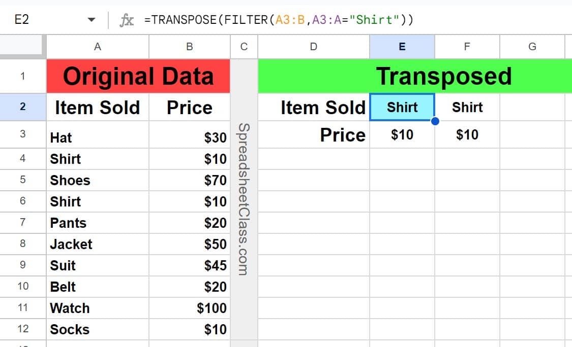
As you can see in the image above, the inventory data is now filtered and only displays “Shirt” items / prices. The same formula that filters the data also transposes the data, which in this case converts columns into rows.
Filter and transpose from rows to columns
Now let’s go over an example where we will filter data and convert from rows to columns.
In this example, the inventory date is entered into rows 2 and 3. What we are going to do is filter the data so that only shirts are displayed, and we will also transpose the data from rows to columns.
The task: Filter the inventory data to show only shirts, and convert from rows to columns
The logic: Filter the range B2:3, where the range B2:2 is equal to the text “Shirt”, and then transpose the result
The formula: The formula below, is entered in the blue cell (A7), for this example
=TRANSPOSE(FILTER(B2:3,B2:2=”Shirt”))
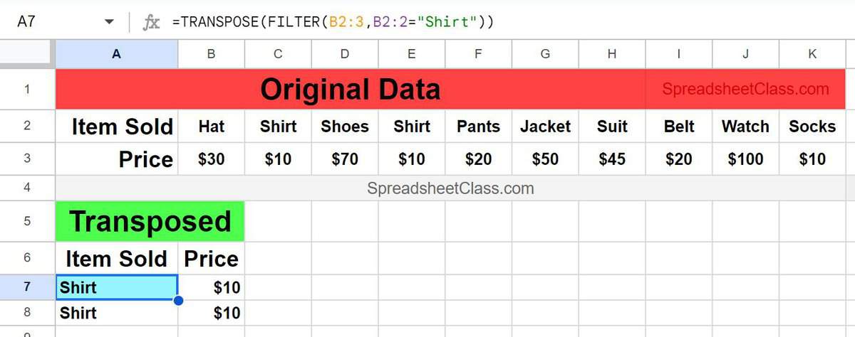
As you can see in the image above, the inventory data is now filtered and only displays “Shirt” items / prices. The same formula that filters the data also transposes the data, which in this case converts rows to columns.