

The TRANSPOSE function is a very useful formula that will allow you to turn rows into columns, or columns into rows, in Google Sheets. If you need to switch the columns and rows in your data, this lesson will show you several ways of using the TRANSPOSE function to do exactly that.
To transpose data (switch columns and rows) in Google Sheets, follow these steps:
- Type "=TRANSPOSE(" or click “Insert” → “Function” → “Array” → “TRANSPOSE”
- Type the range of cells that contains the data that you want to transpose, like this: A1:B10
- Press "Enter" on the keyboard, and your data will be transposed. Your formula will look like this: =TRANSPOSE(A1:B10)
TRANSPOSE formulas in Google Sheets:
Here are the TRANSPOSE formulas that I am going to go over in the examples below.
Transpose column to row
- =TRANSPOSE(A1:A)
Transpose row to column
- =TRANSPOSE(C1:1)
Transpose columns to rows
- =TRANSPOSE(A2:B)
Transpose rows to columns
- =TRANSPOSE(A2:3)
Switch columns and rows for a range of cells
- =TRANSPOSE(A1:I9)
Transpose from another sheet
- =TRANSPOSE('Sheet 1'!A1:I9)
Turn a column into a row
First, let's go over how to turn a single column of data, into a single row, by using the TRANSPOSE function. Later we will do examples with more data, but let's keep it simple for now. The next example will show you the opposite of this example (Rows turned into columns).
Notice in the formula below, that the address of the cell range (A1:A) ends with the letter A, indicating that we are referring to an entire column of data.
The task: Make the vertical list of names, horizontal
The logic: Transpose column A, into row 1, by transposing the range A1:A
The formula: The formula below, is entered in the blue cell (C1), for this example
=TRANSPOSE(A1:A)
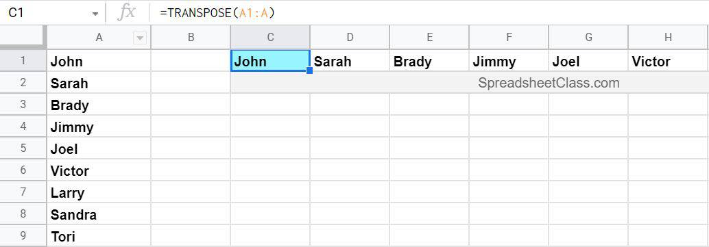
Notice that the names that are listed in column A, are now displayed as a row, in row 1.
Turn a row into a column
Now let's do the opposite of the example above, and turn a single row of data, into a single column, by using the TRANSPOSE function.
Notice in the formula below, that the address of the cell range (A1:1) ends with the number 1, indicating that we are referring to an entire row of data.
The task: Make the horizontal list of item codes, vertical
The logic: Transpose row 1, into column A, by transposing the range C1:1
The formula: The formula below, is entered in the blue cell (A1), for this example
=TRANSPOSE(C1:1)
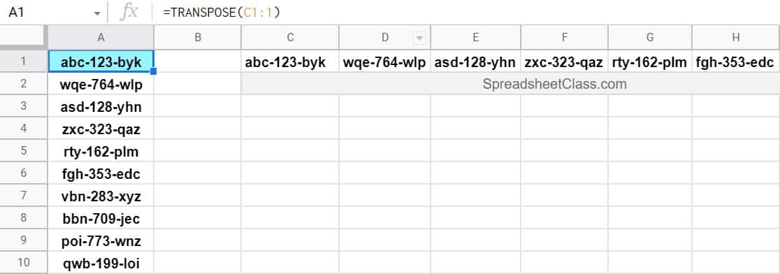
Notice that the item codes that are listed in row 1, are now displayed as a column, in column A.
This content was originally created by Corey Bustos / SpreadsheetClass.com
Turn columns into rows (Multiple Columns / Rows)
Now let's go over a couple examples where we are transposing more than one column / row of data. In this example, we will turn 2 columns of data, into 2 rows.
The task: Transpose the columns of data showing item names and prices, into rows
The logic: Transpose columns A and B, into rows 2 and 3, by transposing the range A2:B
The formula: The formula below, is entered in the blue cell (D2), for this example
=TRANSPOSE(A2:B)
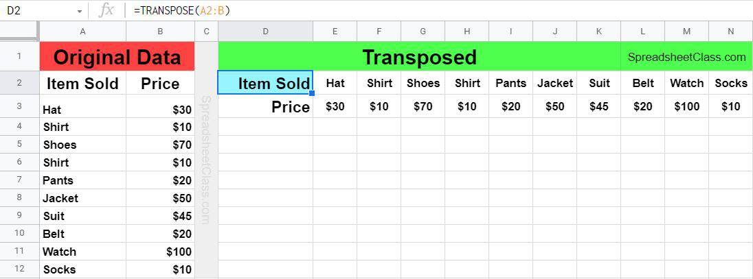
Notice that the item names and prices that are listed in columns A and B, are now displayed as rows, in rows 2 and 3.
Turn rows into columns (Multiple Rows / Columns)
Now let's do the opposite again, and turn 2 rows of data, into 2 columns.
The task: Transpose the rows of data showing item names and prices, into columns
The logic: Transpose rows 2 and 3, into columns A and B, by transposing the range A2:3
The formula: The formula below, is entered in the blue cell (A6), for this example
=TRANSPOSE(A2:3)
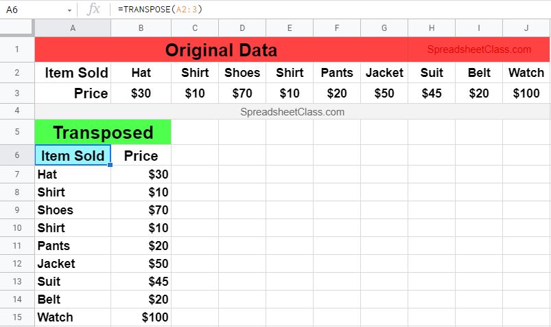
Notice that the item names and prices that are listed in rows 2 and 3, are now displayed as columns, in columns A and B.
Switch rows and columns in a range of cells
In this example, we will use a bigger data set, where we have a range of data that we want to switch the rows / columns of. The image below shows data that displays student grades.
The student names are listed in column A, the Assignment names are listed in row 1, and we want to turn the columns into rows… and the rows into columns…. so that the student names are in row 1, and so that the assignment names are in column A.
The task: Transpose the student grade data, so that columns and rows are switched
The logic: Transpose the data in the range A1:I9
The formula: The formula below, is entered in the blue cell (A11), for this example
=TRANSPOSE(A1:I9)
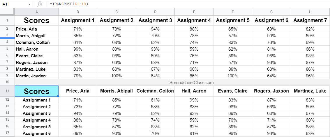
You can see that starting at row 11, the student grade data has been transposed, so that the columns were turned into rows, and vice versa the rows were turned into columns.
Transpose data from another sheet
You might also find the need to transpose data that is on another sheet / tab. This can be done by adding a tab name to your formula. Let's say that we want to refer to the same source data (student grades) from the previous example, but we want to put our formula on a completely different tab.
For this example, let's say that our raw / source data is on a tab named "Sheet 1". You don't have to worry about the name of the tab with the formula, because it is the tab with the course data that we need to refer to with our formula.
As shown below, you can simply add the tab name before typing the cell range, to refer to data from another tab. But remember two important things when referring to other tabs in your formulas.
First, make sure that you put an exclamation point after the tab name, to indicate to Google Sheets that you are referencing a tab. Second, if the tab that you are referring to has a space in its name, you must also include an apostrophe before and after the tab name (as shown below).
The task: Transpose the data from "Sheet 1", into another tab
The logic: Transpose the range A1:I9, from "Sheet 1"
The formula: The formula below, is entered in the blue cell (A1), for this example
=TRANSPOSE('Sheet 1'!A1:I9)
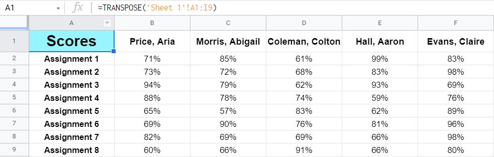
As you can see in the image above, the data from the tab "Sheet 1" has been transposed into a completely different tab.
I hope that this lesson on the TRANSPOSE function makes your work faster and easier!
The Google Sheets TRANSPOSE formula:
Here is a diagram of the TRANSPOSE function, that shows how it works.
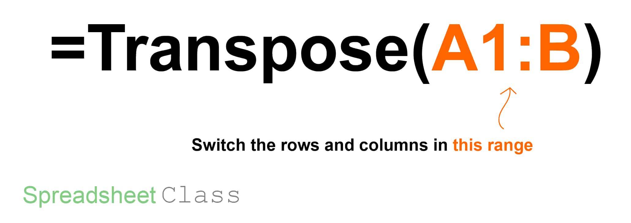
The Google Sheets TRANSPOSE function description:
Syntax:
TRANSPOSE(A2:F9)Formula summary: “Transposes the rows and columns of an array or range of cells.”
Now let's go over some examples of using the TRANSPOSE function, in a variety of ways.
How I use the TRANSPOSE formula in my work
There are a variety of ways that I use the TRANSPOSE function at my job, such as taking a list of vertical dates and listing them horizontally across the top of the sheet when making attendance sheets.
I also use a vertical list of school locations and then apply the TRANSPOSE function to list the locations horizontally across the top of the sheet, such as when I want to provide a list of students who have not recently worked for each location, with one location per column.
Pop Quiz: Test your knowledge
Answer the questions below about the TRANSPOSE formula, to refine your knowledge! Scroll to the very bottom to find the answers to the quiz.
Question #1
Which of the following formulas will turn a row into a column?
- =TRANSPOSE(A1:A)
- =TRANSPOSE(A1:1)
Question #2
Which of these formulas will turn a column into a row?
- =TRANSPOSE(A1:1)
- =TRANSPOSE(A1:A)
Question #3
Which of these formulas will switch columns and rows?
- =TRANSPOSE(A1:Z)
- =TRANSPOSE(A1:J19)
- =TRANSPOSE(A:Z)
- =TRANSPOSE(D1:E99)
- All of the above
Question #4
True or false: The TRANSPOSE function can be used to turn columns into rows, or rows into columns.
- True
- False
Question #5
Which of the following formulas refers to data on another sheet?
- =TRANSPOSE(Sheet1!A1:A)
- =TRANSPOSE('Sheet 1'!A1:A)
- =TRANSPOSE(1!A1:A)
- =TRANSPOSE(A1:A)
- All of the above
- Answers 1, 2, and 3
Answers to the questions above:
Question 1: 2
Question 2: 2
Question 3: 5
Question 4: 1
Question 5: 6