

If you want to remove duplicates and transpose your data with a single formula in Google Sheets, you can do this by combining the UNIQUE function with the TRANSPOSE function.
In this lesson I am going to show you multiple ways of combining these two functions, so that you can remove duplicates and transpose with a single formula.
UNIQUE / TRANSPOSE nested formula
In this lesson we are going to combine two functions together, where the output of one function is used as the criteria for another function. This is commonly referred to as a “nested” function.
For this particular formula combination, it is important to ensure that the correct formula is nested inside of the other.
When using the UNIQUE function and the TRANSPOSE function together, the function that is nested is performed by the spreadsheet first.
The UNIQUE function removes duplicates from rows, and so if we are removing duplicates and converting rows to columns, we want to use the UNIQUE function first to remove the duplicates from the rows, before using the TRANSPOSE function (i.e. the UNIQUE function nested inside of the TRANSPOSE function).
Vice versa, if we are removing duplicates and converting columns to rows, we want to use the TRANSPOSE function to convert the columns to rows, before using the UNIQUE function to remove duplicates from the rows (i.e. the TRANSPOSE function nested inside of the UNIQUE function).
If you want to remove duplicates horizontally, this requires the combination of two TRANSPOSE functions and a UNIQUE function.
First you transpose to convert the rows to columns, then use the UNIQUE function to remove the duplicates vertically, and then use the TRANSPOSE function again to get the data back into rows again.
This lesson focuses on combining the TRANSPOSE and UNIQUE functions, but if you want to learn how to use the functions individually, check out the lessons linked below:
Remove duplicates and convert columns to rows
Let’s go over a simple example of using the TRANSPOSE function and the UNIQUE function together in Google Sheets.
In this example, we have two columns of data… item names in column A, and prices in column B. What we are going to do is remove the duplicates from the data, and then transpose the result so that the columns are converted into rows.
The task: Remove duplicates from the inventory data, and convert the columns to rows
The logic: Remove duplicates from the range A3:B, and then transpose the result
The formula: The formula below, is entered in the blue cell (E2), for this example
=TRANSPOSE(UNIQUE(A3:B))
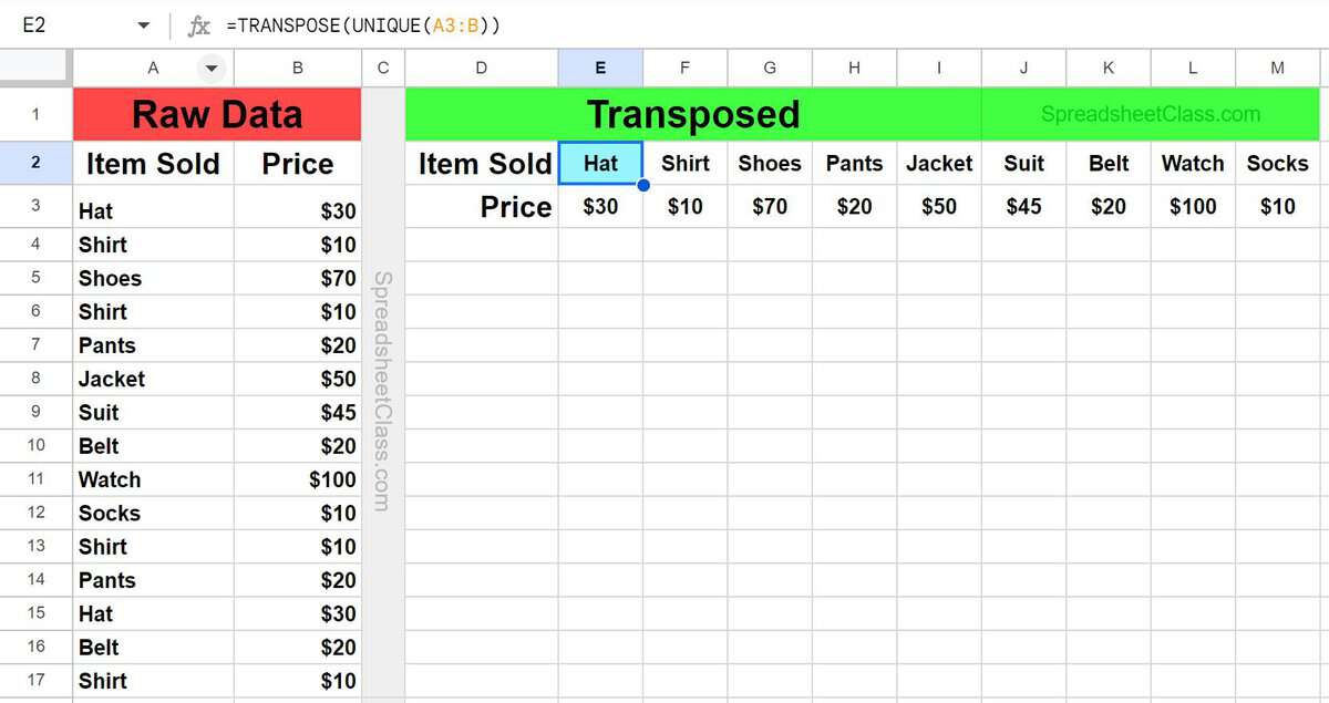
As you can see in the image above, the duplicates from the inventory data have been removed, and the columns have been converted to rows, and this was done by using a single formula.
Remove duplicates and convert rows to columns
In this example, instead of converting from columns to rows, we are going to convert from rows to columns (and remove the duplicates from the data).
Since the original data is listed horizontally, and the UNIQUE function removes duplicates vertically, we need to use the TRANSPOSE function first to convert the rows to columns so that the UNIQUE function works correctly when combined with the TRANSPOSE function.
The task: Convert the rows to columns, and remove the duplicates from the inventory data
The logic: Transpose the range E2:3, and then remove duplicates from the result
The formula: The formula below, is entered in the blue cell (A3), for this example
=UNIQUE(TRANSPOSE(E2:3))
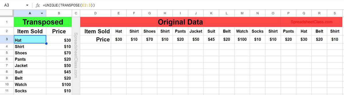
As you can see in the image above, the duplicates from the inventory data have been removed, and the rows have been converted to columns, and this was done by using a single formula.
Remove duplicates horizontally from rows
In this example we are going to combine two TRANSPOSE functions and a UNIQUE function, to remove duplicates horizontally.
First we transpose the data to convert the rows to columns, then use the UNIQUE function to remove the duplicates, and then use the transpose function again to convert back to rows.
In row 1 we have a list of dates, and we want to remove the duplicate dates while keeping the data listed horizontally.
The task: Remove duplicates from the data that is listed horizontally
The logic: Transpose the range B1:1, then remove duplicates from the result, then transpose the result again
The formula: The formula below, is entered in the blue cell (B3), for this example
=TRANSPOSE(UNIQUE(TRANSPOSE(B1:1)))
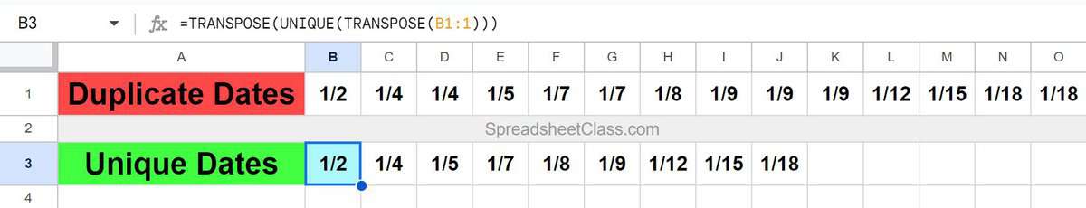
As you can see in the image above, the duplicate dates that are listed in row 1, have been removed.