

If you want to sort and transpose your data with a single formula in Google Sheets, you can do this by combining the SORT function with the TRANSPOSE function. These two functions can be used together in a variety of ways, from sorting data that is converted from columns to rows, sorting data that is converted from rows to columns, and even sorting horizontally.
In this lesson I am going to show you how to combine these two functions, so that you can sort your date and transpose it with a single formula.
SORT TRANSPOSE formulas in Google Sheets:
Sorting horizontally
- =transpose(SORT(transpose(B1:O1),1,true))
Sort and convert from columns to rows
- =TRANSPOSE(SORT(A3:B,2,true))
Sort and convert from rows to columns
- =SORT(TRANSPOSE(E2:3),2,true)
SORT / TRANSPOSE nested formula
In this lesson we are going to combine multiple functions together in a single formula, where one formula is used inside of another function. When we do this this is called a “Nested function”, because we are “nesting” one function inside of another. Another way that this is commonly described is to say that one function is “wrapped” around another function.
This lesson focuses on combining the TRANSPOSE and SORT functions, but if you want to learn how to use the functions individually, check out the lessons linked below:
Sorting horizontally in Google Sheets
Let’s go over a simple example of using the TRANSPOSE function and the SORT function together in Google Sheets.
In this example, we have a list of numbers that are entered horizontally into row 1. What we are going to do is sort the data horizontally in ascending order.
To do this we will need to transpose the data into columns, sort the data, and then transpose it again to convert it back to rows.
This is because the sort function in Google Sheets always sorts vertically, and so we must use the TRANSPOSE function to convert the data to columns, and then back to rows after being sorted. This can be done by using a single formula, as shown below.
The task: Sort the data horizontally
The logic: Transpose the range B1:O1, then sort the result (by column 1 in ascending order), and then transpose the result again
The formula: The formula below, is entered in the blue cell (B3), for this example
=transpose(SORT(transpose(B1:O1),1,true))
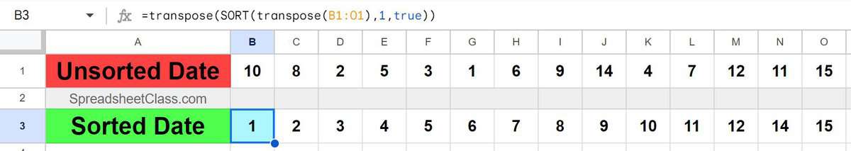
As you can see in the image above, there are unsorted numbers in row 1, and the formula in cell B3 sorts the numbers horizontally.
Sorting data that is converted from columns to rows
In this example, we have a list of items and prices that are entered into columns A and B. What we are going to do is transpose the data so that the columns are converted to rows, and so that the data is sorted in ascending order.
The task: Sort the data by price and then convert the columns to rows
The logic: Sort the range A3:B by column 2 in ascending order, then transpose the result
The formula: The formula below, is entered in the blue cell (E2), for this example
=TRANSPOSE(SORT(A3:B,2,true))
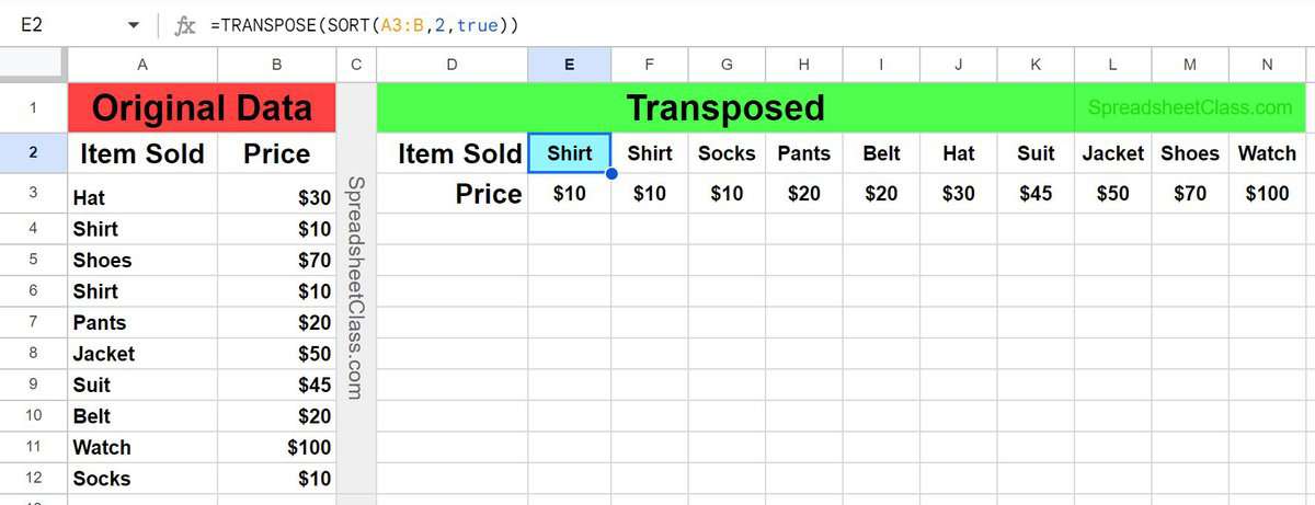
As you can see in the image above, there are items and prices in columns A and B, which are unsorted. The formula in cell E2 sorts the data by price, and then transposes the data from columns to rows.
Sorting data that is converted from rows to columns
In this example, we have a list of items and prices that are entered horizontally into rows 2 and 3. What we are going to do is transpose the data so that the rows are converted to columns, and so that the data is sorted in ascending order.
The task: Convert the rows to columns and then sort the data by price
The logic: Transpose the range E3:2, then sort the result (by column 2 in ascending order)
The formula: The formula below, is entered in the blue cell (A3), for this example
=SORT(TRANSPOSE(E2:3),2,true)
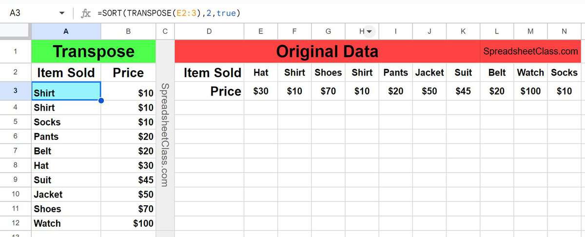
As you can see in the image above, there are items and prices in rows 2 and 3, which are unsorted. The formula in cell A3 transposes the data from rows to columns, and sorts the data by price.