
When you are filtering in Google Sheets, you may sometimes come across an error that says “FILTER has mismatched range sizes”. This is a common error that can be easily fixed by assuring that the references in your filter formula contain the same number of rows. If you happen to be filtering horizontally, then your filter references must contain the same number of columns.
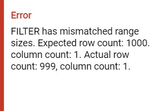
If your filter ranges are not the same size, you will see an error indication appear in the cell where your filter formula is that says “#N/A”, and when you hover over that cell a message will display the following error details:
“FILTER has mismatched range sizes. Expected row count: 1000. column count: 1. Actual row count: 999, column count: 1.”
When your filter formula in Google Sheets displays an error that says “FILTER has mismatched range sizes”, adjust the row number in the ranges of your formula so that both the source data range (data to be filtered), and the criteria column (the column containing values to check against), have the same number of rows. In other words, each range that is referenced in your filter formula should begin and end on the same row.
For example, consider the formulas below. The first formula has mismatched range sizes and will not function properly, but the second and third formula are correct and show how the first formula can be fixed.
Notice that the reference to the source data range begins on row 1, but the reference to the criteria range begins on row 2, which causes the “mismatched range sizes” error.
- =FILTER( A1:C, A2:A=1) This formula will not function
- =FILTER( A1:C, A1:A=1) This is a corrected formula
- =FILTER( A2:C, A2:A=1) This is a corrected formula
Again, if you are filtering horizontally, you must assure that your source range and your criteria range contain the same number of columns.
In this article I will go over several different ways that the “mismatched range sizes” error can appear, and how to fix each of these situations.
If it appears that your references/ranges have the same number of rows but you are still receiving the filter has mismatched range sizes error… then this is likely due to an error related to filtering data from another sheet, where you may have forgotten to include a sheet name in one of your references. I will go over this in detail below, but I wanted to mention it right away because this mistake is a very common cause of the “mismatched range sizes” error.
If you want to learn all about how to use the filter function, check out the article(s) below.
“How to use the Google Sheets FILTER function” (Beginner)
“How to filter based on a list in Google Sheets” (Advanced/Special application)
But in this article we will stick to fixing the mismatched range size error.
Click here to get your Google Sheets cheat sheet
Or click here to take the dashboards course
When the beginning row numbers are mismatched
Below is an example that shows the error that will occur when the beginning row numbers in your filter ranges are not the same.
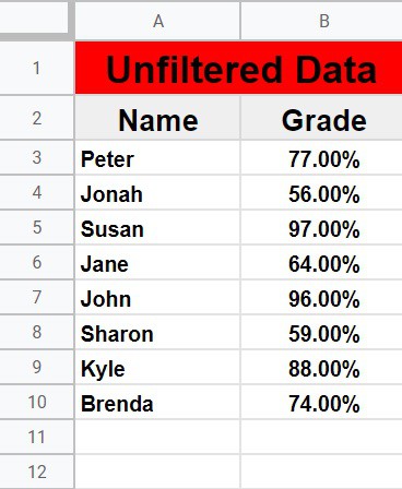
In columns A and B we have a list of student names and their grades. Let’s say that we are trying to filter these names/grades to display only the rows where students received a grade that is greater than 80% (0.8).
In the first image you can see that the filter formula is not working properly, because the reference to the source range begins on row 2 but the reference to the criteria column/range starts on row 3.
This results in the ranges having a different number of rows (i.e. being a different size), and causes the “FILTER has mismatched range sizes” error.
(In the second image you will be able to see the corrected formula with ranges that begin on the same row)
Formula that causes an error: The formula below is entered into cell D3 (blue cell), for this example
=filter(A2:B,B3:B>0.8)

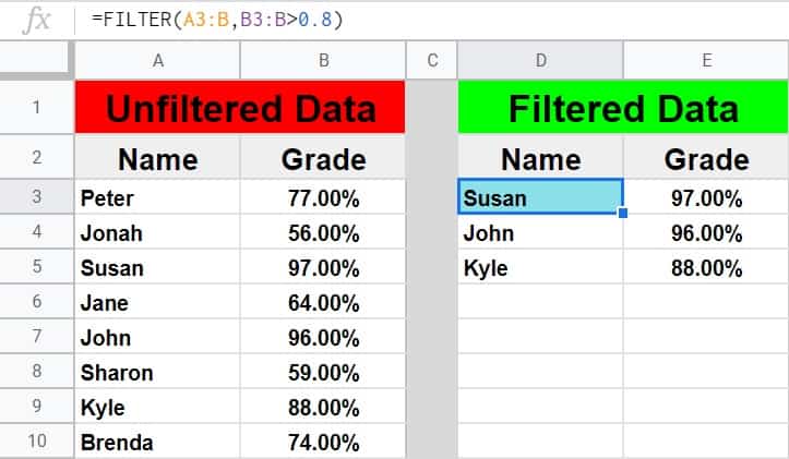
By adjusting one of the references so that both of the ranges begin on row 3, the formula is repaired and will now work properly, as shown below. The formula now displays students who have a grade that is higher than 80%.
Corrected formula: The formula below is entered into cell D3 (blue cell), for this example
=filter(A3:B,B3:B>0.8)
When the ending row numbers are mismatched
The “FILTER has mismatched range sizes” error can also occur when your ending row numbers are not the same, even if you do use the same beginning row number on both ranges.
In the last example we did not specify an ending row number, but now let’s say that we want to designate the ending row of the ranges that in our filter function.
Below, are two formulas. The first formula causes an error because the source range ends on row 10, and the criteria range ends on row 9.
The second formula has been corrected so that both references start and end on the same row, and therefore are the same “size”.
Formula that causes an error:
=filter(A3:B10,B3:B9>0.8)
Corrected formula:
=filter(A3:B10,B3:B10>0.8)
Mismatched range sizes when filtering from another tab
When referring to data that is on another tab, a common mistake is to include the tab name in one of the filter references… but to forget to include it in the other reference. Doing this will cause the “FILTER has mismatched range sizes” error, if the two different sheets that you are referring to (by accident), have a different number of rows.
When this mistake happens it may appear that your references contain the same number of rows when they really do not.
When you are filtering data from another sheet, you must make sure that you include the tab name in your references to both the source range and the filter criteria range.
In this example, we will filter the same data that we used in the previous example with the same criteria (filtering students with grades of more than 80%), but this time the formula and the data to be filtered are on separate sheets.
In the following formula, the tab name “Sheet2” was mistakenly only included in one of the references.
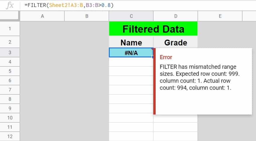
The filter formula is now referring to two different sheets, and since these two sheets contain a different number of rows (and we did not specify an ending row in our references), the ranges in the formula are not the same size, and so the formula will display the “mismatched range sizes” error.
Formula that causes an error: The formula below is entered into cell C3 (blue cell), for this example
=FILTER(Sheet2!A3:B,B3:B>0.8)
Sheet2 (The data to be filtered that is held on another tab):
To correct the formula above, you would simply add the forgotten tab name so that both references refer to the same data set / spreadsheet tab, as shown below.
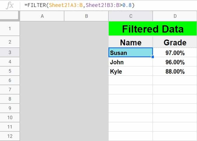
Corrected formula: The formula below is entered into cell C3 (blue cell), for this example
=FILTER(Sheet2!A3:B,Sheet2!B3:B>0.8)
Sometimes you may run into a similar scenario, where you actually meant to remove the tab names in both of your references, but accidentally only removed the tab name in one reference. In this case you would simply remove the remaining tab name so that you were only referring to data on the current tab, as shown below.
Corrected formula (version 2):
=FILTER(A3:B,B3:B>0.8)
Mismatched range sizes when filtering horizontally
As mentioned earlier, if you are filtering horizontally and then you experience the “FILTER has mismatched range sizes” error, you must make sure that your references start and end on the same COLUMN.
When filtering horizontally, it is expected that your ranges will be a different number of rows, but to assure that the horizontal filter ranges are the same size, they must contain the same number of columns.
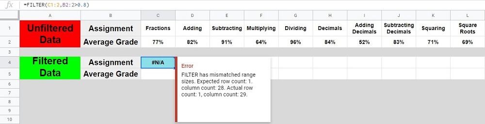
In the example below, in rows 1 and 2 is a list of class assignments and the average grade of each assignment in the class.
The first image/formula shows an attempt to horizontally filter this data, so that only assignments which have an average grade of over 80% (0.8) are displayed.
In the first formula used, the source data range (data to be filtered) begins on column C, where the criteria range/row, begins on column B. This will cause the “FILTER has mismatched range sizes” error, due to the ranges having a different number of columns.
(The second image will show the corrected formula, where the ranges are no longer mismatched)
Formula that causes an error: The formula below is entered into cell C4 (blue cell), for this example
=FILTER(C1:2,B2:2>0.8)
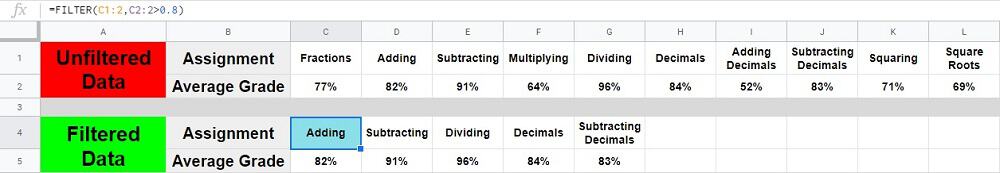
By adjusting one of the references so that both of the ranges specified begin on column C, the formula is repaired and will now work properly, as shown below. The formula now displays assignments that have an average grade higher than 80%.
Corrected formula: The formula below is entered into cell C4 (blue cell), for this example
=FILTER(C1:2,C2:2>0.8)
Now you know exactly how to fix this error when it happens!