

In Google Sheets, you can freeze rows and columns in your spreadsheet, so that a specified amount of rows and/or columns will stay locked in place when you scroll, such as when you want to lock your header rows, or lock a column on the left side of your sheet. This makes it much easier to read your sheets when the data extends beyond the screen view, where you want to be able to always show the row(s) at the top or the column(s) on the left.
In this lesson I am going to show you how to freeze rows, columns, both rows and columns at the same time, and I’ll also show you how to unfreeze rows / columns.
There are two different ways to freeze rows and columns in Google Sheets. You can either use the click and drag method, or you can use the “View” menu, which is the main method that I will use in the examples, but below I will teach you how to use both of these methods.
To freeze rows and / or columns in Google Sheets, follow these steps:
- Select any cell that is in the column / row that you want to freeze (You may also select the entire row or column)
- Click “View” on the top toolbar menu
- Hover your cursor over “Freeze”
- Choose the number of columns or rows that you want to freeze. You can choose to freeze 1 or 2, or if you are freezing more than two columns / rows… you will have the option to freeze “Up to” the cell / row / column that you selected before opening the menu)
Click here to get your Google Sheets cheat sheet
If you freeze a row, the frozen row will remain at the top as you scroll up and down.
If you freeze a column, the frozen column will remain on the left as you scroll left and right.
The two methods for freezing rows and columns in Google Sheets
First, let’s go over the two different ways to freeze rows and columns in Google Sheets. We’ll start with the click and drag method, and then we’ll go over the “View” menu method for the rest of the examples in the lesson.
Click and drag method for freezing rows / columns in Google Sheets
You can use your mouse to freeze rows / columns with the click and drag method, without having to open any menus.
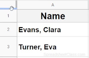
As is shown in the image below, in your Google spreadsheet you will see thick grey lines at the top left of the sheet (Above row 1 and to the left of column A). These thick grey lines / borders can be clicked and dragged downwards to freeze rows, or clicked and dragged to the right to freeze columns.
When you hover your cursor over these thick grey lines, your cursor will turn into a hand when it is in the correct position.
How to freeze rows with the click and drag method
To freeze rows with the click and drag method, find the thick grey horizontal line that is on the left of the sheet, above row 1. Hover your cursor over this thick grey line until the hand appears, click your mouse, hold the click, and then drag your cursor downwards until you have reached the row that you want to freeze, and then release your click. You will see a thick grey line / border across the entire row that is frozen.
How to freeze columns with the click and drag method
To freeze columns with the click and drag method, find the thick grey vertical line that is at the top of the sheet, to the left of column A. Hover your cursor over this thick grey line until the hand appears, click your mouse, hold the click, and then drag your cursor to the right until you have reached the column that you want to freeze, and then release your click. You will see a thick grey line / border across the entire column that is frozen.
“View” menu method for freezing rows / columns in Google Sheets
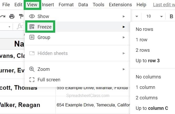
The traditional method for freezing rows and columns in Google Sheets, is by using the “View” menu. As shown below, you can open the “Freeze” menu by clicking “View” on the top toolbar. From this menu you can choose how many rows or columns that you want to freeze.
You will be able to choose between, “No rows”, “1 rows”, “2 rows”, or “Up to row…”
When freezing more than two rows, you must first select the row or column that you want to freeze “Up to” before opening the freeze menu. I’ll tell you more about this in an example later in the lesson.
To freeze rows or columns with the “View” menu method in Google Sheets, click “View” on the top toolbar, then click “Freeze”, and then select how many rows / columns that you want to freeze.
Now let’s go over some detailed examples on how to freeze rows, columns, both, and how to unfreeze.
Unfrozen example data
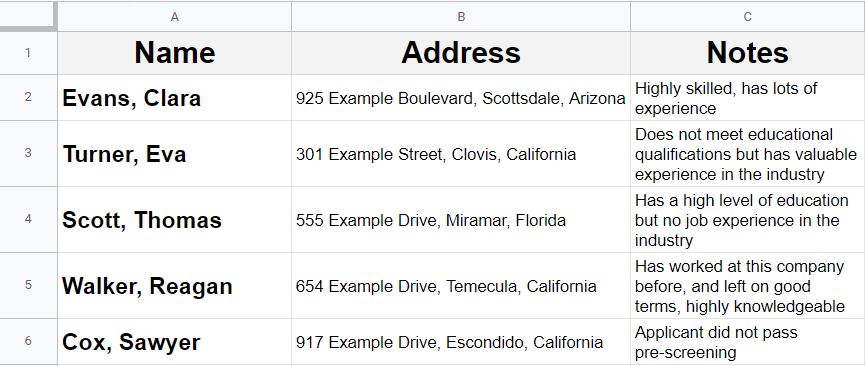
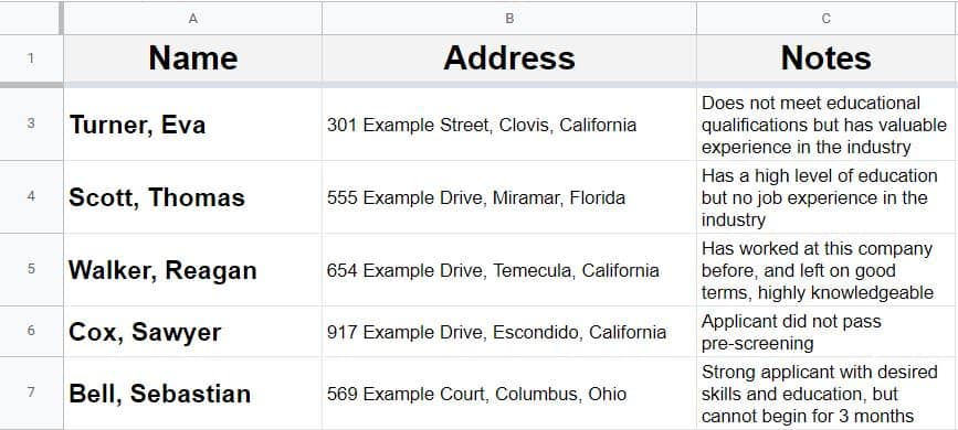
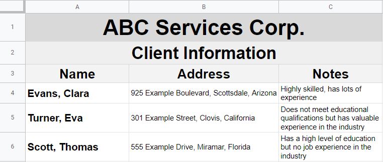
The image below shows data where there are no rows frozen and no columns frozen (before freezing). The example data is a list of potential applicants, their address, and notes on their qualifications. In the examples below we will use this data as an example to freeze rows, columns, both, and more.
How to freeze a row in Google Sheets
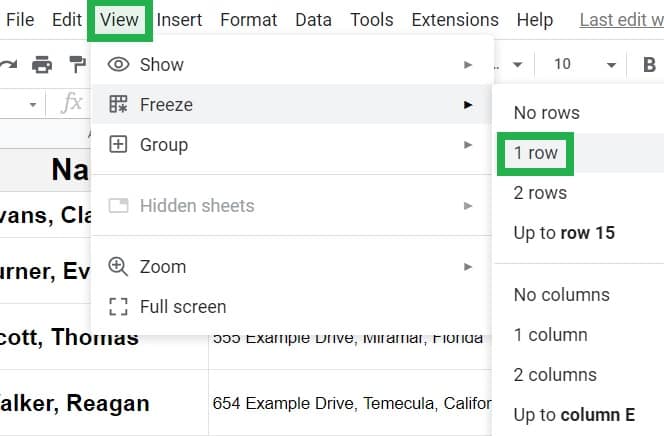
So let’s say that we want to freeze one row, which in this case means freezing the headers, so that when we scroll down the headers stay frozen at the top. To do this we will choose “1 row” from the “Freeze” menu.
To freeze a row in Google Sheets, follow these steps:
- Click “View” on the top toolbar
- Hover your cursor over “Freeze”
- Click “1 row”
Directly below is an image that shows the steps to take to freeze one row in Google Sheets.
The example image below shows the example data after freezing the first row. Notice that there is a thick grey bar / border between the first and second row, indicating that the first row is frozen. Now when we scroll down, the header row will remain frozen at the top.
How to freeze a column in Google Sheets
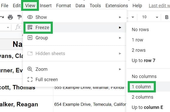
Now let’s freeze a column instead of a row, so that when we scroll right, column A stays frozen on the left. To do this we will choose “1 column” from the “Freeze” menu.
To freeze a column in Google Sheets, follow these steps:
- Click “View” on the top toolbar
- Hover your cursor over “Freeze”
- Click “1 column”
The image directly below shows the steps to take to freeze one column in Google Sheets.
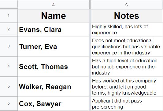
The example image below shows the example data after freezing one column. Notice that there is a thick grey bar / border between the first and second column, indicating that the first column is frozen. Now when we scroll to the right, column A will remain frozen on the left.
How to freeze both rows and columns in Google Sheets
Now let’s freeze both rows and columns, so that when we scroll down the top row is locked on top, and when we scroll right the first column is locked on the left. To do this we will first freeze a row, and then we will freeze a column (Or vice versa, but they must be frozen one at a time).
To freeze both rows and columns in Google Sheets, follow these steps:
- Click “View” on the top toolbar
- Hover your cursor over “Freeze”
- Select the number of rows that you want to freeze
- Repeat the process for columns: Click “View”
- Hover your cursor over “Freeze”
- Select the number of columns that you want to freeze
The example image below shows the example data after freezing a row and a column (Both row 1 and column A are frozen). Notice that there is a thick grey bar / border between the first and second row, as well as between the first and second column, indicating that the first row and the first column are both frozen. Now when we scroll down the first row will remain frozen at the top, and when we scroll right the first column will remain frozen on the left.
How to “Freeze panes” in Google Sheets
“Freeze panes” is an option / button that is available in Excel. To freeze panes in Google Sheets, follow the instructions above to freeze both rows and columns. Remember that selecting the exact cell where you want the rows / columns to be frozen “Up to”, makes it faster to freeze both rows and columns because you only need to select the one cell, rather than selecting a row, and then selecting a column.
How to freeze two rows or two columns in Google Sheets
You can also freeze multiple rows or multiple columns in your Google spreadsheet. To do this we will choose “2 rows” or “2 columns” from the “Freeze” menu. In the next example I’ll show you how to freeze more than 2 rows / columns.
To freeze two rows or two columns in Google Sheets, follow these steps:
- Click “View” on the top toolbar
- Hover your cursor over “Freeze”
- Click “2 rows”, or click “2 columns”
Directly below is an image that shows the steps to take to freeze two rows or two columns in Google Sheets.
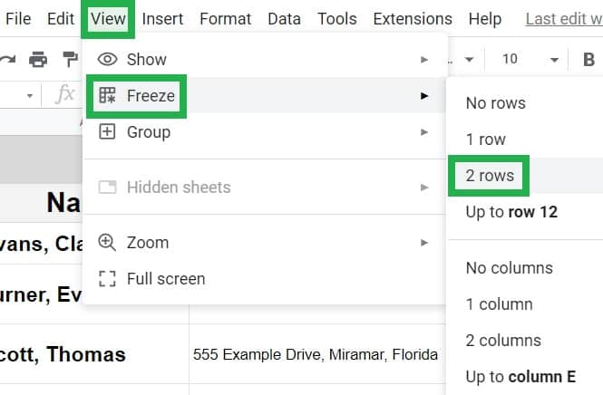
The example image below shows the example data after freezing two rows. Notice that there is a thick grey bar / border between the second and third column, which indicates that the first two rows are frozen. Now when we scroll down, both row 1 and row 2 will remain frozen on the top of your spreadsheet.
This content was originally created by Corey Bustos / SpreadsheetClass.com
How to freeze more than two rows / columns in Google Sheets
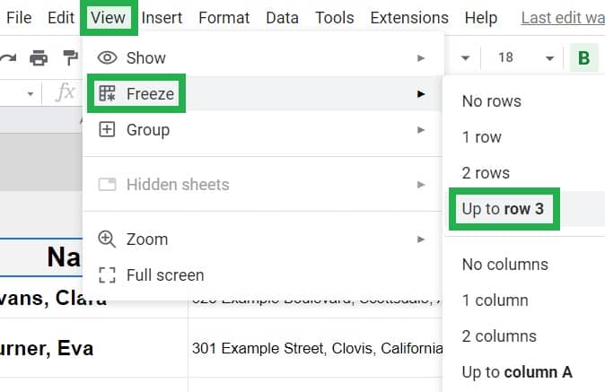
If you want, you can freeze more than 2 rows / columns in a Google spreadsheet. The “Freeze” menu has an option to freeze “Up to” the selected row / column, and so this is how you can freeze 3 or more rows / columns. To do this we will choose “Up to row 3” or “Up to column C” from the “Freeze” menu.
When freezing more than 2 rows or columns in Google Sheets, you’ll first need to select the cell that is within the row / column that you want to freeze, and then the “Freeze” menu will give you the option to freeze “Up to” the selected row / column. If you want, you can select the entire row / column that you want to freeze up to, but you can also simply select the exact cell where you want Google Sheets to freeze up to, and this will allow you to freeze both rows and columns “Up to” the selected cell.
Instead of being numbered, columns in a spreadsheet have letters, where the first column is labeled “A”. So if you want to freeze three columns, this means that you will freeze “Up to” column C.
So if you want to freeze up to row 3, you can select row 3, then click “View”> “Freeze” > “Up to row 3”
If you want to freeze up to column C, you can select column C, then click “View”> “Freeze” > “Up to column C”
Or, you can select cell C3, which will give you the option to freeze “Up to row 3” or “Up to column C” in the “Freeze” menu.
To freeze more than 2 rows or more than 2 columns in Google Sheets, follow these steps:
- Select the cell in your spreadsheet that is in the row / column that you want to freeze
- Click “View” on the top toolbar
- Hover your cursor over “Freeze”
- Click “Up to row 3” / “Up to column C”, (Or whichever row number / column letter that it says when the appropriate cell is selected)
The image directly below shows the steps to take to freeze more than two rows / columns in Google Sheets.
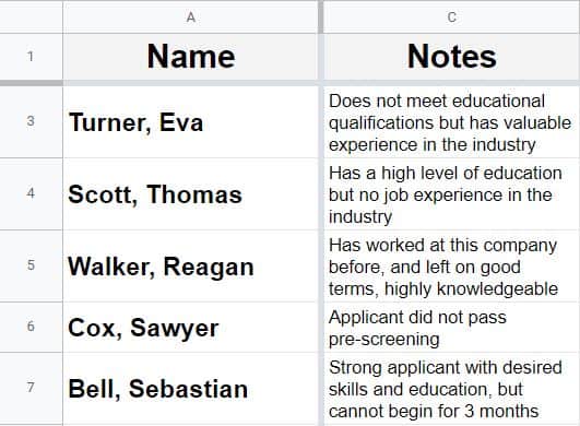
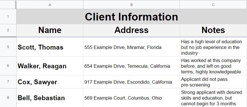
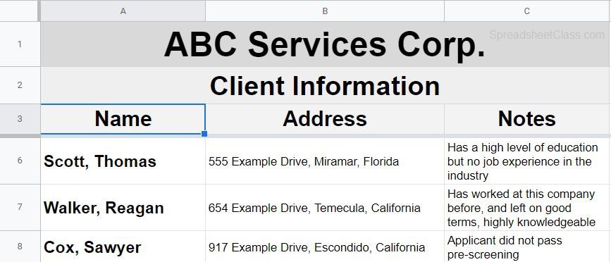
The example image below shows the example data after freezing three rows. Notice that there is a thick grey bar / border between the third and fourth column, which indicates that the first three rows are frozen. Now when we scroll down, rows 1 through 3 will remain frozen on the top of your spreadsheet.
by SpreadsheetClass.com
How to unfreeze columns and rows in Google Sheets
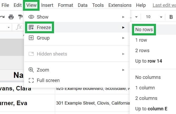
Now that you know how to freeze rows and columns, you’ll want to know how to unfreeze rows or columns in Google Sheets. Unfreezing rows and columns can also be done through the “Freeze” menu. To unfreeze rows and columns, we will choose “No rows” or “No columns” from the “Freeze” menu.
To unfreeze rows and columns in Google Sheets, follow these steps:
- Click “View” on the top toolbar
- Hover your cursor over “Freeze”
- Click “No rows”, or click “No columns”
Directly below is an image that shows the steps to take to unfreeze rows and columns in Google Sheets.
The example image below shows the example data after unfreezing rows / columns. Notice that there is NOT a thick grey bar / border between the rows / columns (which indicates that there are no frozen rows, and no frozen columns).
Now you know how to freeze rows and columns in your Google spreadsheet (as well as how to unfreeze)! This will make your spreadsheets much easier to read and work with, so that you don’t constantly have to scroll up or to the right to see the labels for your rows / columns.