23 Best formulas for Google Sheets (+ Examples)

Welcome to the Google Sheets formula tutorial! Today I am going to help you take your Google Sheets skills to the next level, by teaching you the basics of how to use formulas in Google Sheets, as well as by teaching you how to use the 23 best Google Sheets formulas.

On this page you will find more than just detailed examples of how to use important formulas in Google Sheets… I will also walk you through using each of the formulas in the step by step tutorial.

I will also show you the basics of entering formulas in case you are new to Google Sheets. You will learn how to copy formulas, lock cell references, and more.

These are not just randomly chosen formulas. These formulas were carefully selected by me as the formulas that are the best to know in order to have great skill in Google Sheets. I say this after having created Google spreadsheets professionally for over 7 years. The point of this list isn't to provide a comprehensive list of formulas, or to show you the formulas that I think are "cool"… the point is to teach you a concise list of the most essential formulas that can make the biggest impact in your professional life.

See more Google Sheets templates

The formulas in this lesson are the ones that will allow you to accomplish an incredibly wide variety of tasks and that will make you extremely valuable in the professional world. Learn these formulas and your Google Sheets abilities will be far beyond the average user, and you will have the confidence to build spreadsheets for needed tasks and assignments at your business or your job!

If you want to learn even more formulas and to become more advanced in Google Sheets, check out the additional free resources linked below:

Learn to build dashboards in Google Sheets (4 Dashboards with many more formulas to learn)

More Google Sheets formula lessons (Check out more focused articles on Google Sheets formulas)

Get your Google Sheets formulas cheat sheet

Formula basics in Google Sheets

Before we start the tutorial and go over the detailed examples, let's go over some basics for using formulas in Google Sheets.

How to enter a formula in Google Sheets:

To enter a formula in Google Sheets, click on the cell that you want to enter a formula into, type an equals sign (=), type the desired formula, then press enter. For example, you can enter a cell reference like =B1, or you can use mathematical operators like =2+2 or =A1+3, or you can use functions like the IF function, such as =IF(A1="Complete",1,0)… or the FILTER function such as =FILTER(A1:B,B1:B="Yes").

How to copy / fill formulas in Google Sheets

When using formulas in Google Sheets, you can copy and paste the cells that have formulas in them to quickly copy formulas into other cells without having to enter them over and over again for each new row / column.

To copy / fill formulas in Google Sheets, either copy a cell that has a formula in it and paste it into the desired cell, or use the fill handle to "fill" the formula into the desired cells. The fill handle appears when you hover your cursor at the bottom right of a cell, where you will see your cursor turn into plus sign. Click and hold your mouse when the fill handle appears, and drag your cursor until you have reached end of the range that you want to copy formulas into.

When you copy and paste a cell that has a formula, instead of pasting the value that was in the cell, the formula will be pasted into a new cell, and the cell references will change when doing so. When you copy a formula from left to right, the column reference will change. When you copy a formula from top to bottom, the row reference will change.

For example, let's say that cell A1 has the formula =G3 entered into it. If you copy and paste cell A1, into cell A2… the formula in cell A2 will be =G4. So you pasted the formula one row down, and the cell reference in the formula incremented by one row as well.

Or, if you paste the formula in cell A1 (=G3) one column over instead of one row down… when you copy and paste cell A1 into cell B1… the formula in cell B1 will be =H3. So you pasted the formula one column to the right, and the cell reference in the formula incremented by one column as well.

Read this article to learn more about how to copy formulas and use autofill to fill entire rows / columns with formulas.

How to lock cell references in Google Sheets (Absolute vs. Relative)

If you want you can modify your formulas so that the references do not change when copying them into new cells. This is done by using what is called an absolute reference. By default Google Sheets uses relative references which change when copied / pasted, as described above, but you can use a dollar sign ($) to lock the references in the formula.

You can choose to lock only columns, or only rows, or both. The dollar sign is entered before the column letter if you want to lock the column references, like this =$Z3
For the formula above, the column references will not change when you copy the formula from left to right, but the row references will change when you copy the formula from top to bottom.

The dollar sign is entered before the row number if you want to lock the row references, like this =Z$3
For the formula above, the row references will not change when you copy the formula from top to bottom, but the column references will change when you copy the formula from left to right.

Google Sheets formula examples and tutorial

Each of the formula examples on this page are connected to the same source / raw data, so instead of having a completely new scenario for each example, we will keep building our new formulas on the same data set / scenario which will make things simple for me and for you.

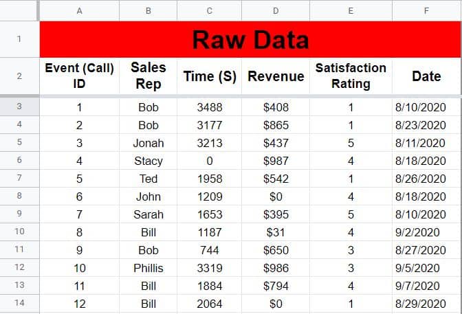
So the data that we will be using is data that shows revenue earned on sales calls by a variety of sales representatives. We will do a wide variety of things with this data as you learn each of the formulas below.

IF function in Google Sheets:

IF formula breakdown (How it works): With the IF function, you can tell Google Sheets to do one thing if a specified criteria is met, and to do something else if the criteria is not met. In other words, the IF function allows you to create an IF / THEN statement. "If TRUE, do this… if FALSE, do this instead."

Formula summary: “Returns one value if a logical expression is TRUE and another if it is FALSE.”

To use the IF function in Google Sheets, enter a logical expression, then specify the value if TRUE, and then specify the value if FALSE, like this: =IF(D3>0,"Yes","No")
The formula above tells Google Sheets, "If D3 is greater than zero, then display the text "Yes", if D3 is not greater than zero, display the text "No" ".

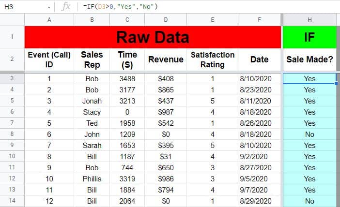
Here is a detailed example of using the IF function. We will use an IF formula to indicate whether or not a sale was made on each call, based on whether or not revenue was earned on each call.

The task: Display the text "Yes" if revenue is greater than zero, and display the text "No" if revenue is not greater than zero

The logic: If cell D3 is greater than 0, then display the word "Yes". If D3 is not greater than 0, display the word "No"

The formula: The formula below, is entered in the blue cell (H3), for this example

=IF(D3>0,"Yes","No")

SORT function in Google Sheets

SORT formula breakdown (How it works): With the SORT function, you can tell Google Sheets to sort a specified range, in a specified order, and you can also choose which column to sort by.

Formula summary: “Sorts the rows of a given array or range by the values in one or more columns.”

To use the SORT function in Google Sheets, enter the range of data that you want to sort, then specify the column that you want to sort by, and then specify the order that you want to sort in (TRUE = Ascending and FALSE = Descending, like this: =SORT(A3:F,2,true)
The formula above tells Google Sheets, "Sort the range A3:F, by the second column, and in ascending order".

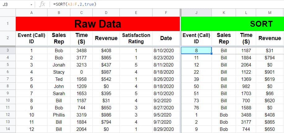
Here is a detailed example of using the SORT function. We will use a SORT formula to sort the sales data by sales rep name.

The task: Sort the sales data in columns A through F, by the name of the sales reps, from A to Z

The logic: Sort the range A3:F, sort by the second column, and sort in ascending order

The formula: The formula below, is entered in the blue cell (J3), for this example

=SORT(A3:F,2,true)

Read this article to learn more about how to use the SORT function in Google Sheets.

Cell reference formula in Google Sheets

Cell references are the easiest type of formula to use, and also one of most used formulas. You will have many times where you want to simply "Refer" to data, where you want the value from one cell to also be the value that is in another cell.

Cell reference formula breakdown (How it works): With a cell reference formula, you can tell Google Sheets to display / pull the value from one cell, into another cell of your choice.

To refer to a cell in Google Sheets, type an equals sign, and then type the address of the cell that you want to refer to / reference, like this: =A2
The formula above tells Google Sheets, "Display the contents of cell A2".

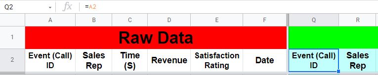
Here is a detailed example of using a cell reference. We are going to use cell references to refer to the headers in the sales data, so that the headers appear in another location.

The task: Display the header text from the raw sales data in columns Q through V

The logic: In cell Q2, display the contents of cell A2. In cell R2, display the contents of cell B2… and so on.

The formula: The formula below, is entered in the blue cell (Q2), for this example, and is copied into the cells to the right, through cell V2

=A2

Referring to another sheet in Google Sheets

Just like ordinary cell reference formulas… formulas that refer to data on another sheet are incredibly important to learn.

Sometimes you might want to refer to data that is on another sheet / tab, and so I will show you how to refer to single cells from another sheet, and I'll also show you how to pull data from another sheet by referring to an entire range with the ARRAYFORMULA function (we will go over this function in more detail in another example).

Pulling data from another sheet formula breakdown (How it works): When pulling data from another sheet, you can tell Google Sheets to display the contents of a chosen cell or a chosen range of cells, from a specified tab.

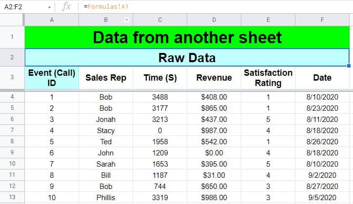
To reference data from another sheet in Google Sheets, type an equals sign, then type the name of the tab that you are referencing, and then type the cell address that you want to refer to, like this: ='Formulas'!A1
The formula above tells Google Sheets, "Display the contents of cell A1, from the "Formulas" tab".

To pull data from a range on another sheet, type an equals sign, type ARRAYFORMULA, type the name of the tab that you are referencing, and then type the cell range that you want to refer to, like this: =ARRAYFORMULA('Formulas'!A2:F12)
The formula above tells Google Sheets, "Display the contents of the range A2:F12, from the "Formulas" tab".

Here is a detailed example of pulling data from another sheet. We are going to refer to a single cell from another sheet, as well as a range of cells from another sheet.

The task: Pull the raw sales data from the "Formulas" tab, onto a different sheet

The logic: In cell A2, display the contents of cell A1 from the "Formulas" tab. Starting at cell A3, display the contents of the range A2:F12 from the "Formulas" tab (By using the ARRAYFORMULA function)

The formulas: The formulas below, are entered in the blue cells (A2 & A3), for this example

='Formulas'!A1

=ARRAYFORMULA('Formulas'!A2:F12)

FILTER function in Google Sheets

FILTER formula breakdown (How it works): With the FILTER function, you can tell Google Sheets to filter a specified range, by a specified column, by using a specified condition / criteria.

Formula summary: “Returns a filtered version of the source range, returning only rows or columns which meet the specified conditions.”

To use the FILTER function in Google Sheets, enter a source range, then specify the column to filter by, and then specify the criteria, like this: =FILTER(A3:F,H3:H="Yes")
The formula above tells Google Sheets, "Filter the range A3:F where H3:H is equal to the word "Yes" ".

Here is a detailed example of using the FILTER function. We will use a FILTER formula to display only the rows where the sales rep made a call.

The task: Filter the sales data to show only the calls where a sale was made

The logic: Filter the range A3:F, where column H (H3:H) is equal to the text "Yes"

The formula: The formula below, is entered in the blue cell (Q3), for this example

=FILTER(A3:F,H3:H="Yes")

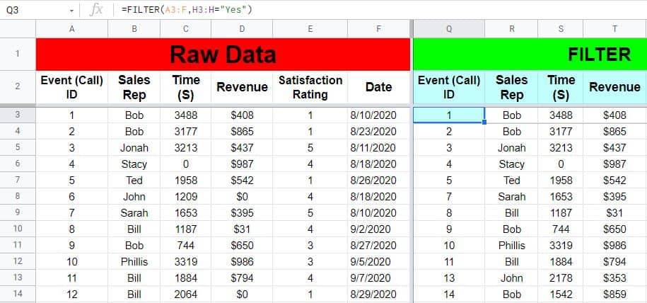
In this example we used column H as the criteria column for the FILTER function, where we had previously entered an IF function into column H. If we wanted, instead of only showing rows where column H equaled "Yes", we could have displayed only the rows that had revenue greater than zero to get the same result, like this: =FILTER(A3:F,D3:D>0)

Read this article to learn more about how to use the FILTER function in Google Sheets.

ARRAYFORMULA function in Google Sheets

The ARRAYFORMULA function is an incredibly useful function, with many different uses. You can use it by itself to reference entire ranges of cells with a single formula, of you can use it combined with other functions such as the SPLIT function, to extend the functionality of formulas throughout an entire range by using a single formula. You can also use the "&" operator with ARRAYFORMULA to combine / concatenate columns (I will show you more examples of using ARRAYFORMULA, within the other examples below).

ARRAYFORMULA formula breakdown (How it works): With the IF function, you can tell Google Sheets

Formula summary: “Enables the display of values returned from an array formula into multiple rows and/or columns and the use of non-array functions with arrays.”

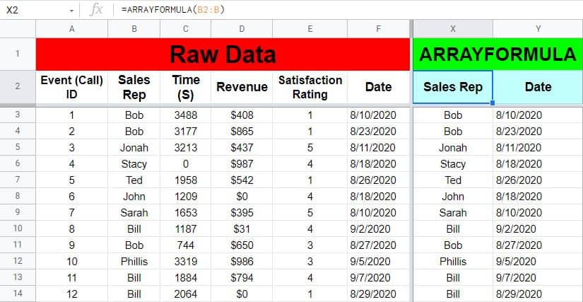
To use the ARRAYFORMULA function in Google Sheets, enter a range of cells that you want to refer to, as the reference for the ARRAYFORMULA function, like this: =ARRAYFORMULA(B2:B)
The formula above tells Google Sheets, "Display the contents of the range B2:B".

Here is a detailed example of using the ARRAYFORMULA function. We will use an ARRAYFORMULA formula to

The task: Display the contents in the cells from column B

The logic: Use ARRAYFORMULA to refer to the values in the range B2:B

The formula: The formula below, is entered in the blue cell (X2), for this example, and is copied into cell Y2

=ARRAYFORMULA(B2:B)

Read this article to learn more about how to use the ARRAYFORMULA function in Google Sheets.

UNIQUE function in Google Sheets

UNIQUE formula breakdown (How it works): With the UNIQUE function, you can tell Google Sheets to remove the duplicates from a specified range of cells.

Formula summary: “Returns unique rows in the provided source range, discarding duplicates. Rows are returned in the order in which they first appear in the source range.”

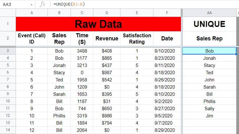
To use the UNIQUE function in Google Sheets, enter a range of cells that you want to remove duplicates from, as the reference for the UNIQUE function, like this: =UNIQUE(B3:B)
The formula above tells Google Sheets, "Remove the duplicates from the range B3:B".

It is important to note that when the UNIQUE function determines whether or not a certain row is a duplicate, the formula considers the entire row of the range that is entered into the formula. So if you only refer to a single column, the UNIQUE function will only look at the data within that single column to check for duplicates in each row. But if you refer to multiple columns, the values in both columns must be the same as the values from another row, for the UNIQUE function to consider the row / entry a duplicate (You can learn more about this in the article linked below.)

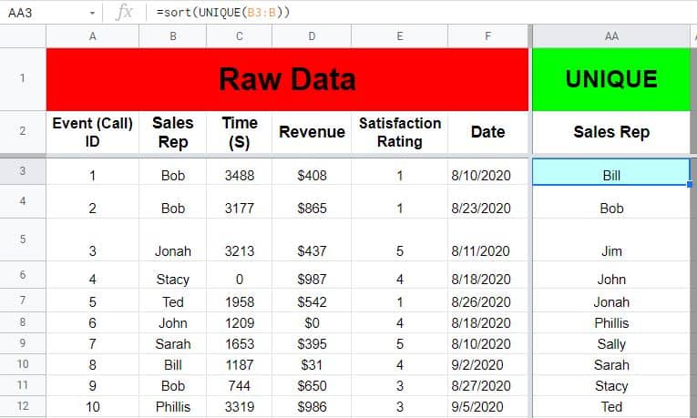
Here is a detailed example of using the UNIQUE function. We will use a UNIQUE formula to display a list of all sales representatives.

The task: Remove the duplicate names from column B, to display a list of sales reps

The logic: Remove the duplicate values from the range B3:B

The formula: The formula below, is entered in the blue cell (AA3), for this example

=UNIQUE(B3:B)

Read this article to learn more about how to use the UNIQUE function in Google Sheets.

Using nested formulas in Google Sheets

Nested formulas are essential for being able to work with data on a professional level in Google Sheets. There are many functions to work with in Google Sheets, but there are many more ways that you can combine these function to create what is called a "Nested" function.

In this example we are going to combine the SORT function with the UNIQUE function, so that the UNIQUE results are also sorted.

Combining functions together entails "Nesting" one function inside of another function, or in other words "Wrapping" one function around another function.

Nested formula breakdown (How it works): With a nested formula, you can tell Google Sheets to apply the functionality of one formula, to the results of another formula. The function that is nested is performed first, and then the formula that is "Wrapped" around the nested function is applied to the result of the nested function.

To use a nested formula in Google Sheets, enter one formula, and then refer to that formula as the source range / data for another function, like this: =sort(UNIQUE(B3:B))
The formula above tells Google Sheets, "Sort the results / output of the UNIQUE function".

Here is a detailed example of using a nested formula. We will use a nested formula to sort the results of the UNIQUE function.

The task: Sort a unique list of sales reps

The logic: Remove the duplicates from the range B3:B with the UNIQUE function, and then sort the result with the SORT function

The formula: The formula below, is entered in the blue cell (AA3), for this example

=sort(UNIQUE(B3:B))

COUNTIF function in Google Sheets

COUNTIF formula breakdown (How it works): With the COUNTIF function, you can tell Google Sheets to count the number of times that a specified criteria is met.

Formula summary: “Returns a conditional count across a range.”

To use the COUNTIF function in Google Sheets, enter the range that contains the data to check / test against your criteria, then enter the criteria that you want to count, like this: =COUNTIF(B:B,AA3)
The formula above tells Google Sheets, "Count how many times that the value in cell AA3 is found in column B".

Here is a detailed example of using the COUNT function. We will use a COUNTIF formula to count how many calls are listed for each sales rep in the raw data.

The task: Count the total number of calls placed by each sales rep

The logic: Count how many times that the value entered into cell AA3, is found in column B (B:B)

The formula: The formula below, is entered in the blue cell (AC3), for this example, and is copied into the cells below it

=COUNTIF(B:B,AA3)

Note that in this example, as well as several of the following examples, we are not referring directly to the raw data, but we are referring to the names of the sales reps / other data that was generated in a previous example.

SUMIF function in Google Sheets

SUMIF formula breakdown (How it works): With the SUMIF function, you can tell Google Sheets to sum a specified range, where a specified range is equal to a specified criteria.

Formula summary: “Returns a conditional sum across a range.”

To use the SUMIF function in Google Sheets, enter the range to test / check against your criteria, then enter the criteria, and then enter the range that you want to sum when the criteria is met, like this: =SUMIF(B:B,AA3,D:D)
The formula above tells Google Sheets, "Sum column D, where the value in cell AA3 is found in column B".

Note that the "Sum Range" is optional, and if you do not enter it, Google Sheets will default to summing the criteria range.

Here is a detailed example of using the SUMIF function. We will use a SUMIF formula to show the total revenue for each sales rep.

The task: Display the total revenue earned for each sales representative

The logic: Sum column D (D:D), for each row where the value in cell AA3 is found in column B (B:B)

The formula: The formula below, is entered in the blue cell (AE3), for this example

=SUMIF(B:B,AA3,D:D)

AVERAGEIF function in Google Sheets

AVERAGE formula breakdown (How it works): With the AVERAGEIF function, you can tell Google Sheets to average a specified range, where a specified range is equal to a specified criteria.

Formula summary: “Returns the average of a range depending on criteria.”

To use the AVERAGEIF function in Google Sheets, enter the range to test / check against your criteria, then enter the criteria, and then enter the range that you want to average when the criteria is met, like this: =AVERAGEIF(B:B,AA3,E:E)
The formula above tells Google Sheets, "Sum column E, where the value in cell AA3 is found in column B".

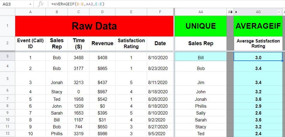
Here is a detailed example of using the AVERAGEIF function. We will use an AVERAGEIF formula to find the average satisfaction rating for each sales rep.

The task: Find the average satisfaction rating for each sales representative, considering all sales calls

The logic: Average column E (E:E), for each row where the value in cell AA3 is found in column B (B:B)

The formula: The formula below, is entered in the blue cell (AG3), for this example, and is copied into the cells below it

=AVERAGEIF(B:B,AA3,E:E)

Count non-blank cells in Google Sheets

There are many cases where you may need to count how many cells in your sheet are not blank. There is a very easy way to do this with the COUNTIF function, while using the "Not" operator / symbol, which looks like this: <>

Count non-blank cells formula breakdown (How it works): With the COUNTIF function, you can tell Google Sheets to count all of the cells in a specified range that are not blank.

To count non-blank cells in Google Sheets, enter a source range, then specify the criteria, like this: =COUNTIF(AA3:AA12,"<>")
The formula above tells Google Sheets, "Count how many cells are not blank in the range AA3:AA12".

Here is a detailed example of counting non-blank cells. We will use the COUNTIF formula to count how many sales reps there are.

The task: Count how many sales representatives there are

The logic: In the range AA3:AA12, count how many cells are not blank / not empty

The formula: The formula below, is entered in the blue cell (AI3), for this example

=COUNTIF(AA3:AA12,"<>")

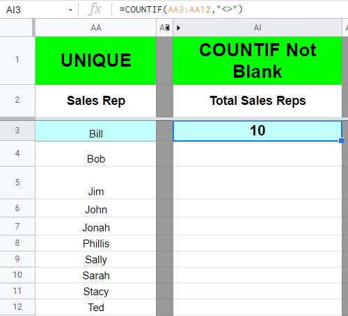
As you can see in the image above, there are 10 sales representatives. But remember that we got this answer by referring to the list of unique sales reps. If we had referred to the raw data, the COUNTIF function would have given us the total number of entries in the report.

COUNTUNIQUE function in Google Sheets

COUNTUNIQUE formula breakdown (How it works): With the COUNTUNIQUE function, you can tell Google Sheets to count the unique / non-duplicate values in a specified range.

So remember the statement from above that said if we had counted non-blank cells in the raw data, such as column B (Sales Reps), the formula would have given use the total number of entries. But if we want we can use the COUNTUNIQUE function, to do the same thing as using the UNIQUE function and then counting non-blank cells, all in one formula. So if we refer to column B with the COUNTUNIQUE function, we will get the same answer as in the example above (10 Sales Reps).

Formula summary: “Counts the number of unique values in a list of specified values and ranges.”

To use the COUNTUNIQUE function in Google Sheets, enter the source range of the data that you want to count unique values in, like this: =COUNTUNIQUE(B3:B)
The formula above tells Google Sheets, "Count the unique values in the range B3:B".

Here is a detailed example of using the COUNTUNIQUE function. We will use a COUNTUNIQUE formula to count the total number of unique sales reps.

The task: Count how many unique sales reps there are by referring to the raw data

The logic: In the range B3:B, count the unique / non-duplicate values

The formula: The formula below, is entered in the blue cell (AI6), for this example

=COUNTUNIQUE(B3:B)

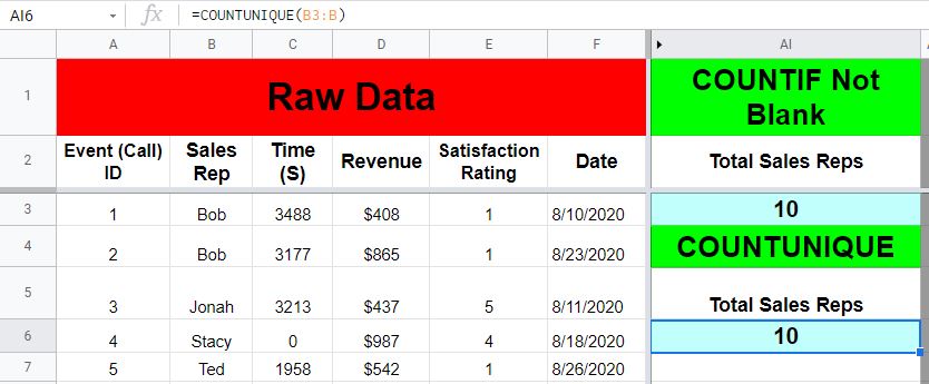
In the image above you can see that the COUNTUNIQUE function gave us the same answer as the formula that count non-blank cells, by referring to the raw data.

SUM function in Google Sheets

SUM formula breakdown (How it works): With the SUM function, you can tell Google Sheets to add up all of the numerical values in a specified range.

Formula summary: “Returns the sum of a series of numbers and/or cells.”

To use the SUM function in Google Sheets, specify the range that contains the values that you want to sum / add together, like this: =SUM(AE3:AE12)
The formula above tells Google Sheets, "Sum all of the numbers in the range AE3:AE12".

Here is a detailed example of using the SUM function. We will use a SUM formula to calculate the total revenue earned for all sales calls combined. If we wanted, we could sum column D to get this number, but we are going to sum column AE, which contains the total revenue per sales rep. Either way will give the same answer.

The task: Calculate the total revenue earned, considering all sales calls

The logic: Sum the values that are in the range AE3:AE12, with the SUM function

The formula: The formula below, is entered in the blue cell (AK6), for this example

=SUM(AE3:AE12)

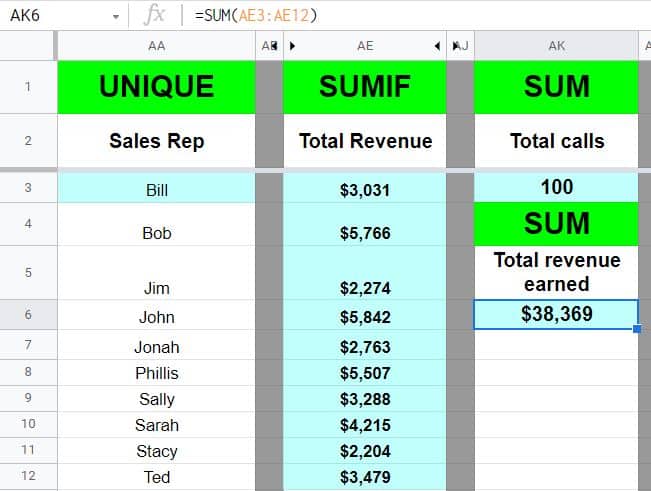
Notice that in the image above, there is another formula entered into cell AK3, that shows the total number of calls. This formula sums column AC, which displays the total calls per sales rep. The formula to enter into cell AK3 is =SUM(AC3:AC12)

AVERAGE function in Google Sheets

AVERAGE formula breakdown (How it works): With the AVERAGE function, you can tell Google Sheets to average the numerical values in a specified range.

Formula summary: “Returns the numerical average value in a dataset, ignoring text.”

To use the AVERAGE function in Google Sheets, specify the range that contains the values that you want to average, like this: =AVERAGE(AC3:AC12)
The formula above tells Google Sheets, "Average the numbers in the range AC3:AC12".

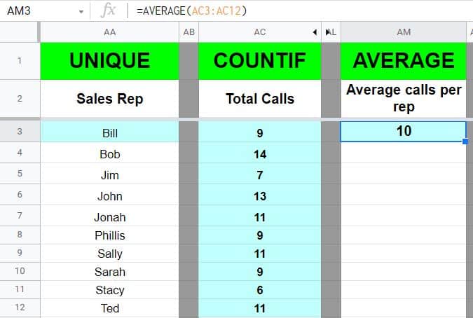
Here is a detailed example of using the AVERAGE function. We will use an AVERAGE formula to find the average number of calls per sales rep.

The task: Calculate the average number of calls that each sales rep placed

The logic: Find the average the numbers in column AC (AC3:AC12) with the AVERAGE function

The formula: The formula below, is entered in the blue cell (AM3), for this example

=AVERAGE(AC3:AC12)

Using mathematical operators in Google Sheets

Mathematical formula breakdown (How it works): Some of the most useful and simple formulas that you can use in Google Sheets, are mathematical formulas. You can do math by using mathematical operators, such as asterisk (*), forward slash (/), plus sign (+), and minus sign (-).

Google Sheets also has functions that will allow you to do math, such as "PRODUCT", but it is much more common and more simple to use operators as shown in this example.

To do math in Google Sheets, separate two values with a mathematical operator, like this: =AK6/AK3
The formula above tells Google Sheets, "Divide cell AK6, by cell AK3".

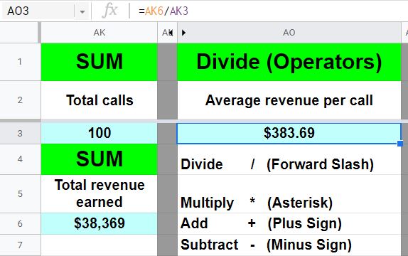
Here is a detailed example of using mathematical operators. We will use a forward slash (/) to divide, and find the average revenue per call.

The task: Calculate the average revenue that was earned on each call, considering all calls

The logic: Divide the value that is in cell AK6 (Total Revenue), by the value that is in cell AK3 (Total Calls). Divide "total revenue" by "total calls".

The formula: The formula below, is entered in the blue cell (AO3), for this example

=AK6/AK3

Read this article to learn more about how to do math in Google Sheets.

Mathematical operators can also be used with the ARRAYFORMULA function, to perform mathematical operations on entire columns, as shown in the formula below.

=ARRAYFORMULA(A1:A/B1)

The formula above would add the value in cell B1, to each of the values / rows in column A

VLOOKUP function in Google Sheets

VLOOKUP formula breakdown (How it works): With the VLOOKUP function, you can tell Google Sheets to display the value of a specified column, in the same row where a specified search key is found in a specified search range.

Formula summary: “Vertical lookup. Searches down the first column of a range for a key and returns the value of a specified cell in the row found.”

To use the VLOOKUP function in Google Sheets, enter a search key, then specify the range to consider for the search, and then specify the column number that you want to return, like this: =VLOOKUP(AR3,A:B,2)
The formula above tells Google Sheets, "Search for the value in cell AR3, through the range A:B, and display the value from the second column in the same row that the search key is found in".

Here is a detailed example of using the VLOOKUP function. We will use a VLOOKUP formula to display the name of a sales rep when searching for a Call ID.

The task: Match the name of the appropriate sales rep by looking up a Call ID (25). i.e. Find the name of the sales rep that was on Call #25.

The logic: Search for the number 25 through range A:B, and display the value that is in the second column (B), from the same row that the search key (25) is found in. Use the VLOOKUP function to do this.

The formula: The formula below, is entered in the blue cell (AR4), for this example

=VLOOKUP(AR3,A:B,2)

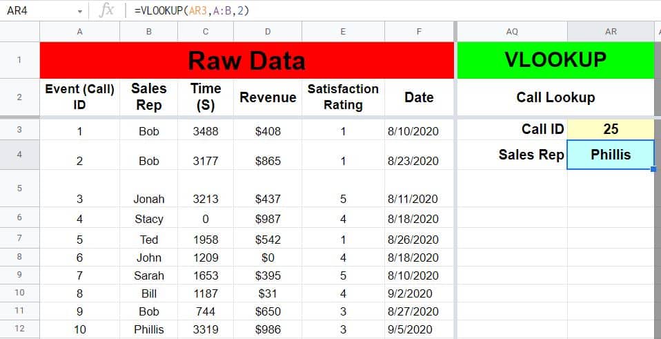
As you can see in the image above, when searching for the Call ID "25", the VLOOKUP function shows us the name "Phillis", which is in the second column of the search range (A:B), in the same row that the number 25 is found in.

TRANSPOSE function in Google Sheets

TRANSPOSE formula breakdown (How it works): With the TRANSPOSE function, you can tell Google Sheets to turn columns into rows, or rows into columns.

Formula summary: “Transposes the rows and columns of an array or range of cells.”

To use the TRANSPOSE function in Google Sheets, enter a range that you want to switch the rows / columns of, like this: =TRANSPOSE(A2:F2)
The formula above tells Google Sheets, "Transpose the row in the range A2:F2, into a column".

Here is a detailed example of using the TRANSPOSE function. We will use a TRANSPOSE formula to create a vertical list of the column headers from the raw data.

The task: Display a vertical list of the column headers from the raw data

The logic: Transpose the range A2:F2

The formula: The formula below, is entered in the blue cell (AT3), for this example

=TRANSPOSE(A2:F2)

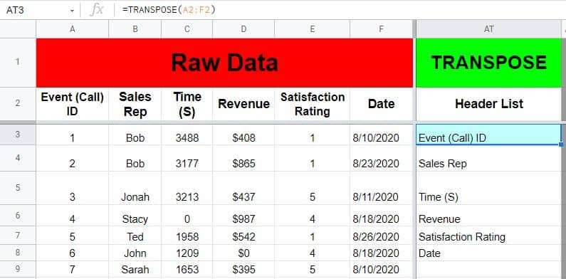
In this example we used the TRANSPOSE function to turn a single row into a single column. The TRANSPOSE function can be used on larger ranges of data as well, where the source range has multiple rows / columns. In this case the function will turn rows into columns, and columns into rows, all at once.

Read this article to learn more about how to use the TRANSPOSE function in Google Sheets.

SPLIT function in Google Sheets

SPLIT formula breakdown (How it works): With the SPLIT function, you can tell Google Sheets to split a string of characters into different cells, where the string is split at / by a specified character (or string of characters).

Formula summary: “Divides text around a specified character or string, and puts each fragment into a separate cell in the row.”

To use the SPLIT function in Google Sheets, enter a cell address that contains the value to be split, then specify the character(s) to split by, like this: =SPLIT(AV2," ")
The formula above tells Google Sheets, "Split the string of characters that is in cell AV2, each time there is a space".

When using a space as the character to split by, the SPLIT function will split each word of a sentence into individual cells.

Here is a detailed example of using the SPLIT function. We will use a SPLIT formula to split the following text / words into individual cells: "Split Text"

The task: Split the text that is entered into a single cell, into individual cells. Split the string "Split Text", where each word is in its own cell.

The logic: Split the value that is in cell AV2, each time there is a space, with the split FUNCTION

The formula: The formula below, is entered in the blue cell (AV3), for this example

=SPLIT(AV2," ")

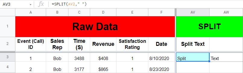
Notice that in cell AV2 the words "Split Text" are together in a single cell, but after using the SPLIT function, the text is split into individual cells… where the word "Split" is in cell AV3, and the word "Text" is in cell AW3.

The split function is a function that can be used with the ARRAYFORMULA function. For example, if you had a column of First / Last names, and you wanted to split the column of names into two separate columns that showed first names in one column and last names in another, you can do this with a single formula by using ARRAYFORMULA and the SPLIT function, in a nested formula, as shown below.

=ARRAYFORMULA(SPLIT(A1:A," "))

The formula above would split the names in column A, into first and last names.

CONCATENATE function in Google Sheets

CONCATENATE formula breakdown (How it works): With the CONCATENATE function, you can tell Google Sheets to combine strings of text / characters.

Formula summary: “Appends strings to one another.”

To use the CONCATENATE function in Google Sheets, enter a string of text or a cell that contains a string, then type a comma, and then specify the next cell / string to append, like this: =CONCATENATE(AV3," ",AW3)
The formula above tells Google Sheets, "Combine the string in cell AV3 with the string in cell AW3, and put a space between them".

Note that the ARRAYFORMULA function can do the same thing as the CONCATENATE function, as shown below.

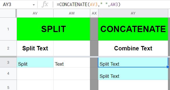
Here is a detailed example of using the CONCATENATE function. We will use a CONCATENATE formula to combine words in separate cells, into a single cell.

So in the last example, we split the words "Split Text" into separate cells… but in this example we are going to combine them again, into a single cell.

The task: Combine the words that are in separate cells (Split / Text), into a single cell

The logic: Combine the contents of cell AV3, with the contents of cell AW3, and put a space between them, by using the CONCATENATE function

The formulas: The formula below, is entered in the blue cell (AY3), for this example

=CONCATENATE(AV3," ",AW3)

=ARRAYFORMULA(AV3&" "&AW3)

Notice that the ARRAYFORMULA function entered into cell AY4, does the same thing as the CONCATENATE function entered into cell AY3.

TODAY function in Google Sheets

Formula breakdown (How it works): With the TODAY function, you can tell Google Sheets to display the current date in a spreadsheet cell.

Formula summary: “Returns the current date as a date value.”

To use the TODAY function in Google Sheets, enter the following formula into a spreadsheet cell: =TODAY()
The formula above tells Google Sheets, "Display today's date".

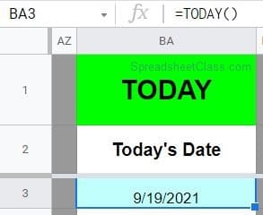
Here is a detailed example of using the TODAY function.

The task: Display today's date

The logic: Use the TODAY function to display the current date in cell BA3

The formula: The formula below, is entered in the blue cell (BA3), for this example

=TODAY()

SUBSTITUTE function in Google Sheets

Formula breakdown (How it works): With the SUBSTITUTE function, you can tell Google Sheets to replace a specified string of text / characters, with another specified string of characters.

Formula summary: “Replaces existing text with new text in a string.”

To use the SUBSTITUTE function in Google Sheets, enter a logical expression, then specify the value if TRUE, and then specify the value if FALSE, like this: =SUBSTITUTE(AY3,"Text","Strings")
The formula above tells Google Sheets, "In cell AY3, replace "Text", with "Strings".

Here is a detailed example of using the SUBSTITUTE function.

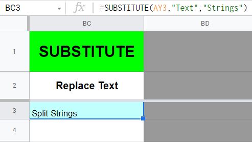
The task: Change the text "Split Text", into the text "Split Strings"

The logic: In cell AY3, replace "Text", with "Strings", by using the SUBSTITUTE function, so that the cell contents "Split Text", turns into the following: "Split Strings"

The formula: The formula below, is entered in the blue cell (BC3), for this example

=SUBSTITUTE(AY3,"Text","Strings")

This content was originally created by Corey Bustos / SpreadsheetClass.com

Notice that in cell BC3, where the cell contents previously said "Split Text", after using the SUBSTITUTE function, the cell contents now say "Split Strings".

IMPORTRANGE function in Google Sheets

Formula breakdown (How it works): With the IMPORTRANGE function, you pull data from one Google Sheets file, into another Google Sheets file, automatically.

Formula summary: “Imports a range of cells from a specified spreadsheet.”

To use the IMPORTRANGE function in Google Sheets, enter the URL or Sheet ID of the Google Sheet that you want to pull data from, then specify the Tab Name + Range that you want to pull data from, like this: =IMPORTRANGE("Sheet ID / URL","'Formulas'!a2:f")
The formula above tells Google Sheets, "Pull data from the specified URL / Google Sheet, from the "Formulas" tab, from range A2:F".

Note that when using the IMPORTRANGE function, after entering the formula, you will have to click on the cell that contains the formula, and click the blue button to give access to the data that you are trying to pull.

You can either specify the entire URL, or the Sheet ID of the Google spreadsheet that you are pulling data from. The sheet ID can be found within the URL, as shown in the image below. I prefer to use the entire URL because it makes it easy to copy and paste into a browser if I need to trace down the source sheet for data that I am pulling from.

If you want, for practice, you can simply use the URL / Sheet ID from the same sheet you are already working in. Although the function will be pulling data from the same file as opposed to its normal use of pulling data from other files… this will allow you to follow along with the example and see that you have setup the formula properly. After that you can change the formula URL / Tab name / Range to see that it works for pulling data from other files.

Here is a detailed example of using the IMPORTRANGE function. We will use an IMPORTRANGE formula to pull raw data from the "Formulas" tab. Again we will be pulling data from the same file to make things easy, but the process is the same as pulling data from another file.

The task: Pull the raw data from columns A through F, from the "Formulas" tab, from the specified URL

The logic: Use the IMPORTRANGE function to pull data from the range A2:F, from the "Formulas" tab, using the URL from the same sheet, or another sheet.

The formula: The formula below, is entered in the blue cell (BE2), for this example

=IMPORTRANGE("Sheet ID / URL","'Formulas'!a2:f")

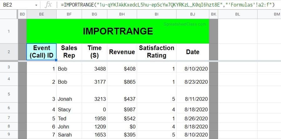
Notice that the raw data from the range A2:F, now displays in the range BE:BJ.

Now you know the best and most important formulas in Google Sheets! Scroll to the top to see linked resources for taking your Google Sheets knowledge to the next level.