

There are many different options for coloring cells in Google Sheets that will allow you to make your spreadsheet visually appealing and easy to read.
It may sound obvious, but cell color is something that I see people at work forgetting to take advantage of all the time. I personally give lots of thought in how I color the cells in my spreadsheets, to provide visual separation that makes things easy to read, or to color code certain items, or to apply nice professional branding to spreadsheets.
To color a cell or a range of cells in Google Sheets, do the following:
- Select the cell or range of cells that you want to change the color of
- Then click the fill color button/menu found in the toolbar
- Then select the color that you want
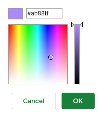
If you want, you can click “Custom…” after opening the color menu, so that you can choose the exact color that you want.
After selecting the desired cells to color, click "Fill Color"

Select desired default color
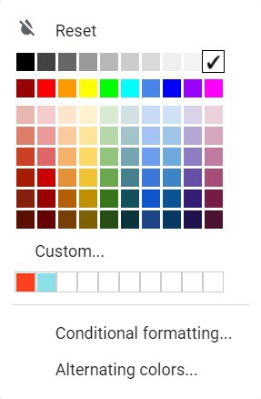
(Optional)- Click "Custom…" and then select a custom color
In this article I will show you how to color cells in Google Sheets, and I will also show you how to change the color of text, change border color, and also how to apply alternating row colors.
For the examples below, if needed, refer to the images above that show how to open the color palette and select default color, or custom colors.
The color selection options will be the same for coloring text and borders, except that they are held under a different toolbar menu.
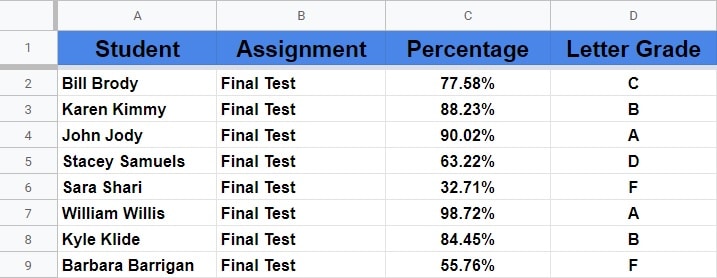
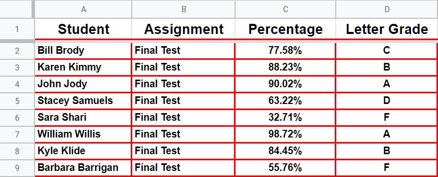
In the examples, we will be using the same set of data (student assignment grades) to color in a variety of ways.
How to change cell color in Google Sheets
First, let's change the color of a single cell. When referring to changing the color of a cell itself, we are talking about changing the background color of that cell.
To color a cell in Google Sheets, select the cell that you want to color, open the "fill color" menu, then select the color that you want.
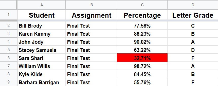
Notice that in this example, in cell C6, the assignment grade is 32.71%. Let's say that we want to manually mark this cell red, to make it stand out.
To do this simply click/select cell C6, then open the "Fill Color" menu, then select the color red.
(See the top of this article for visual instructions on selecting color from the palette)
How to change the color of a range of cells
Now let's select multiple cells to color, or in other words we will select a range of cells to color.
To color a range of cells in Google Sheets, select the range of cells that you want to color, open the "fill color" menu, then select the color that you want.
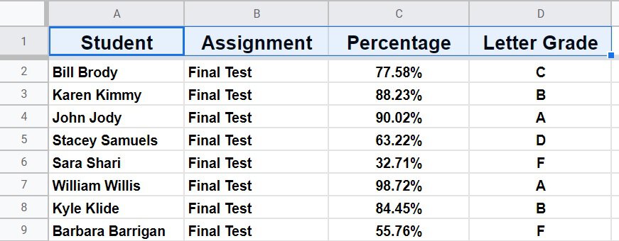
In this example we will color the range A1:D1 to make the cells in the header stand out. (Notice that only 4 cells are selected here, as opposed to a whole row being selected which we will go over in the next example)
To do this simply select the range A1:D1, then open the fill color menu as previously demonstrated at the top of the article, and select your desired color (cornflower blue in this example).
To select a range of cells (A1:D1), use one of the following methods to select multiple cells:
- Click and drag the cursor from Cell A1 to cell D1, or…
- Hold the "ctrl" key on the keyboard while individually clicking the cells A1, B1, C1, and D1 or…
- Select cell A1 and then while holding the "shift" key on the keyboard, then press the right arrow key on the keyboard 3 times or…
- Select cell A1 and then while holding the "shift" key on the keyboard, click cell D1
How to change row color in Google Sheets
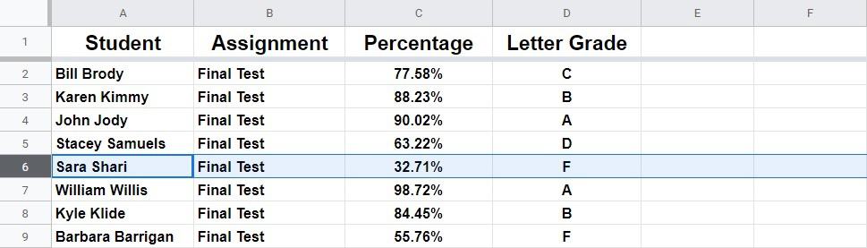
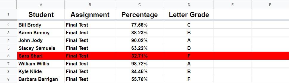
To change row color in Google Sheets, click on the number itself on the very left of the row that you want to color, which will select the entire row of cells, then open the "Fill color" menu, and then select the color that you want.
In this example we will color row 6 red.
To do this click on the number "6" on the far left of row 6 to select the entire row, open the "Fill color" menu, and then select the color that you want.
How to change column color in Google Sheets
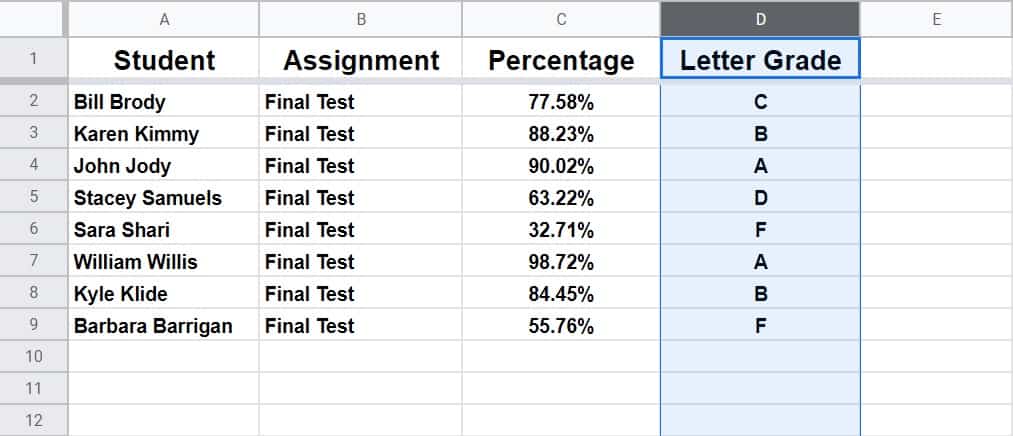
To change column color in Google Sheets, click on the letter itself at the top of the column that you want to color, which will select the entire column of cells, then open the "Fill color" menu, and then select the color that you want.
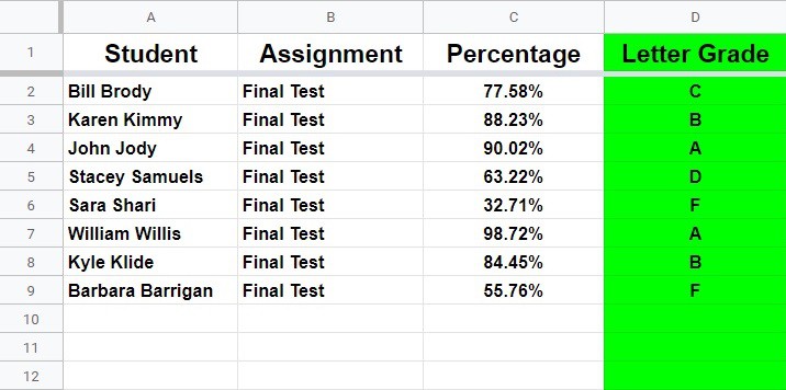
In this example, we will color column D green, to make the "letter grade" column stand out.
To do this click on the letter "D" on the top of column D to select the entire column, open the "Fill color" menu, and then select the color that you want.
How to alternate row color in Google Sheets
In some cases you may want to color every other row in your spreadsheet, and this can be done in a much easier way than by manually selecting every other line before coloring.
To alternate row color in Google Sheets, select the range that you want to apply alternating colors to, open the "Fill color" menu, click "Alternating colors…", customize the options for styling, and then click "Done".
(If you want, you can also select the header or even the entire sheet)
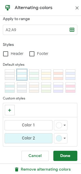
If you prefer, you can also open the alternating colors menu without selecting a range first, and then type the range that you want to color in the "Apply to range" field. If you select the range before opening the menu, you will see that the "Apply to range" field will already be filled in.
When styling alternating colors, you can select a default style, or you can also specify which colors that you want to use.
You can also select whether or not you want there to be a special color for the header/footer.
If the color does not begin on the row that you want, for example if you want the color to be on even rows instead of odd rows… you can either adjust your source range by one row, or flip the colors assigned to "Color 1" and "Color 2" in the menu.
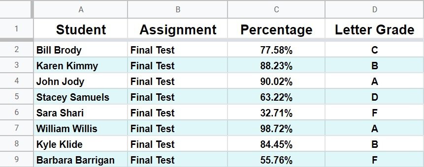
In this example the range that we are applying alternating colors to is A2:D9.
How to remove alternating colors
At the bottom of this article I will go over how to remove color from cells in general, but let's go over how to remove alternating colors specifically.
To remove alternating colors in Google Sheets, select the range that has color to remove, open the alternating color menu while (open the "Fill color" menu, then click "Alternating colors"), and then click "Remove alternating colors".
Alternating row color is a format that will remain even if you click "Reset" in the color menu. If you manually color a cell that already has alternating colors, you will see the color change to what you manually select, but the alternating color format will still be applied in the background unless you click "Remove alternating colors" as described above.
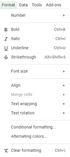
To remove alternating colors, after selecting the range that you want to remove color from, you can also open the "Format" menu, and then click "Clear formatting".
I'll go over clearing formatting more below, but for now, note that this will remove ALL formatting from a cell.
Alternate column OR row color with conditional formatting in Google Sheets
Another way to use alternating colors is the use conditional formatting. With this method you will be able to alternate row colors, or if needed you will also be able to alternate column colors.
To apply alternating colors with conditional formatting, use any of the 4 formulas below, in the "Format cells if…" options, under the "Custom formula is" drop-down selection:
- =ISEVEN(ROW())
- =ISODD(ROW())
- =ISEVEN(COLUMN())
- =ISODD(COLUMN())
Conditional formatting is an amazingly useful tool that allows you to format cells based on their contents, and the following is just one of the many ways that you can use conditional formatting in Google Sheets.
Like in the last example, here you can either select the range to color first, or you can type it into the "Apply to range" field in the conditional formatting menu.
To open the conditional formatting menu do either of the following:
- Click the "Format" menu, and the click "Conditional formatting…" or…
- Open the "Fill color" menu, and click "Conditional formatting…"
Then select "Custom formula is" from the drop-down menu under the "Format cells if…" options.
Then use one of the formulas described below, depending on your preference/situation.
The formula below will color even rows:
=ISEVEN(ROW())
The formula below will color odd rows:
=ISODD(ROW())
The formula below will color even columns (B, D, F, etc…):
=ISEVEN(COLUMN())
The formula below will color odd columns (A, C, E, etc…):
=ISODD(COLUMN())
If you want you can choose your own color from the formatting style options, and you can select other formatting options to apply to the cells/rows/columns that your conditional formatting rules apply to.
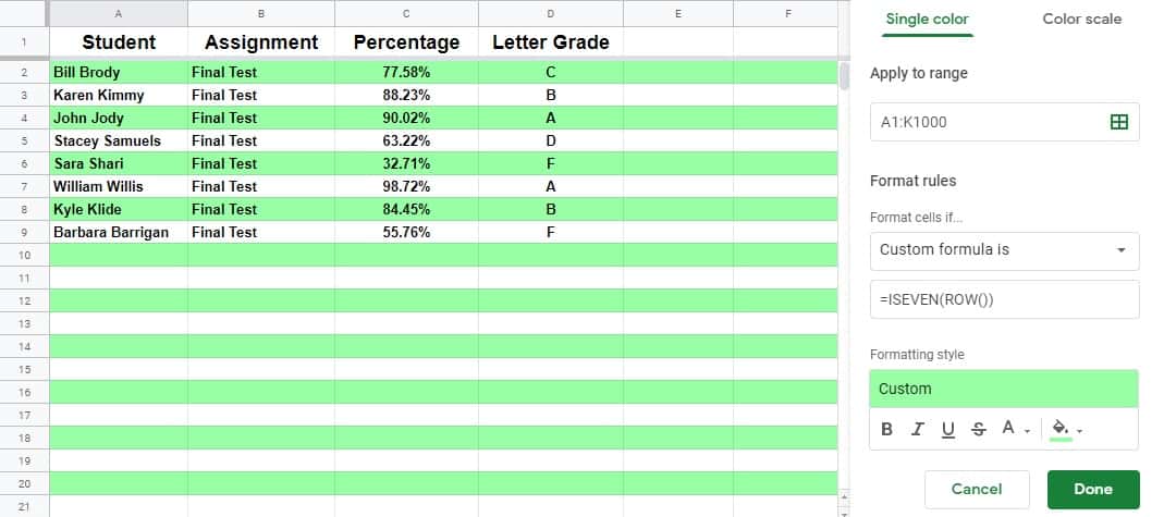
The example below uses the formula =ISEVEN(ROW()) to color even rows. The range that the rule / color is applied to is A1:K1000
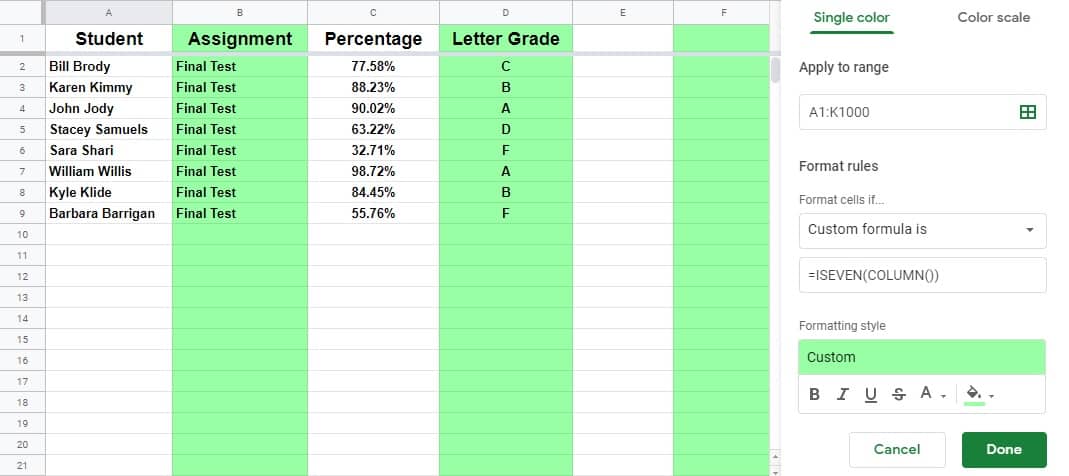
This example uses the formula =ISEVEN(COLUMN()) to color even columns. The range that the rule / color is applied to is A1:K1000
To remove this type of alternating color that is applied with conditional formatting, you can do either of the following:
- Open the conditional formatting menu and click "Remove rule" (Trash can symbol) to remove the conditional formatting or…
- Select a range, then click "Format, then click "Clear formatting". But note that this method will remove ALL formatting
How to change text color in Google Sheets
Changing the color of text in your spreadsheet is almost the exact same as changing cell background color, except that you must click a different menu to begin with.
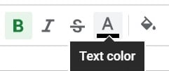
To change text color in Google Sheets, select the range of cells that contain the text/values that you want to color, open the "Text color" menu, and then select the color that you want.
Like with changing the color of cells, when changing text color you can select a single cell, a range, a row, or a column… and then change the color to anything that you want.
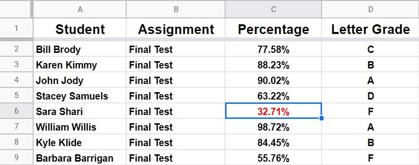
In this example we are going to color the text in cell C6 red, rather than changing the color of the cell itself, which we did in the first example.
To do this simply select cell C6, then open the "Text Color" menu, and then select the color red.
How to change border color in Google Sheets
You may also find certain situations where you want to change the color of borders in Google Sheets.
Most likely you will want to do this to simply change the shade of grey/black of borders, but in this example I have used the color red to make the lines stand out.
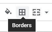
To change border color in Google Sheets, you must first select the cell or range of cells that you want to modify, then open the "Borders" menu in the toolbar, then open the "Border color" menu, and then you must apply the type of border that you want to see. If you do not apply / re-apply borders, changing the line color will not take effect.
In this example we are going to color the borders of the cells in the range A2:D9 red. (I have also made the lines thicker here to make the color stand out more in the image)
To do this, select the range A2:D9, open the "Borders" menu, and then open the "Border color" menu, and then select the color red.
Copying and pasting color/formatting
In some situations you can simply copy and paste a colored cell, to color another cell location.
This will replicate any formatting and contents into the pasted cell location, beyond just color… so this is only usable in some situations, but I have often used this as a quick method to copy cell color (or white space) to another place very quickly.
How to remove color from cells in Google Sheets
Removing color from cells, is in most cases almost exactly the same process as adding color.
To remove color from cells in Google Sheets, select the cells/rows/columns that you want to remove color from, open the "Fill color" menu, and then click "Reset". You can also simply click the color white if you prefer.
Another way to remove color from cells, including any color that is applied through conditional formatting or alternating colors, is to clear the formatting of selected cells by doing the following:
- Select the cells that you want to clear color/formatting from
- Click the "Format" menu in the toolbar
- Click "Clear formatting"
(Using "Clear formatting" will clear ALL/ANY formatting from the cells)
Now you know lots of different ways to color your spreadsheets, so that you can make your finished work visually appealing and very easy to read!