5 formulas that combine columns in Excel

There are a variety of different ways to combine columns in Excel, and I am going to show you five different formulas that you can use to combine multiple columns into one. Three of these formulas will combine columns horizontally, and two of them will combine columns vertically.

Directly below are quick instructions for combining columns, but also look further below for detailed examples, as well as additional ways of combining columns.

This lesson will teach you how to combine columns in Excel, but check out this article if you want to learn how to combine columns in Google Sheets.

Using arrays in Excel

Notice that some of the formulas we are using in this lesson use what are called "arrays". An array formula is entered into a single cell but applies the formula to a range of cells. If you are using an older version of Excel, when using "arrays", you will need to hold "Ctrl" and "Shift" on the keyboard, and then press "Enter" when entering your array formulas. This is called a CSE (Control / Shift / Enter) formula, and is also sometimes called a "Legacy" array, as opposed to newer "Dynamic" arrays that do not require this extra step.

After doing the Ctrl / Shift / Enter method, your formula will be wrapped in curly brackets { }. Notice that the two formulas below will perform the same task, but were simply entered differently, the bottom formula being the "CSE" formula.

=A3:A10&B3:B10

{=A3:A10&B3:B10}

Combine columns in Excel (Horizontal)

First I am going to show you how to combine columns in Excel horizontally.

If you have two columns that you would like to combine the contents of, where the values of the cells in each row are to be combined together horizontally, then there are a few simple ways of doing this:

• The first method (using the "&" operator / ampersand), will allow you to not only combine/merge two columns horizontally, but will also allow you to separate the contents with specified values/ strings of text, and will also allow you to combine more than two columns if you wish
• The second method (using the CONCATENATE function), will allow you to combine the contents of two or more columns horizontally. The CONCATENATE function is almost identical to CONCAT, and I will mention more about this function below.

Both of these methods can be used to combine individual cells, without having to use the ARRAYFORMULA function.

Using the AND operator / ampersand (&) to combine columns

First I will show you the most common and functional way of combining columns horizontally in Excel. In this example we will combine first and last names into a single column.

By using the "&" operator you will be able to combine multiple columns in Excel, and you will also be able to specify values and strings of text that you would like to attach to the column combination.

To combine the data from individual cells in Excel (Such as first & last name), follow these steps:

1. Type an equals sign, and then type the address for the first cell that you want to combine with, such as A3
2. Type an ampersand (&)
3. Type the address of the another cell that you want to combine with, such as B3
4. Press enter on the keyboard. The full formula will look like this: =A3&B3
5. Copy / fill down the formula to use it on the entire column, or turn the cell references into range references to turn the formula into an array

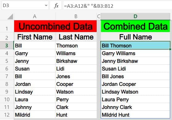
In this first example we have a list of first names in one column, and last names in another column… and we want to combine these columns horizontally so that in each row the full combined name is displayed as a single text string, in a single column.

We will also put a separating space between the contents that are combined in this example. This is accomplished by using quotation marks with a space between them i.e. (" ") in the array formula (shown below).

The task: Horizontally combine the "first name" column with the "size" column, and put a space between the contents… so that the full name is displayed in a single column.

(Where the contents of the cells in each row are combined into a single text string separated by a space)

The logic: Horizontally combine the contents of the cells in the range A3:A12, with the contents of the cells from the range B3:B12, and add a space between the text/contents from the combined columns

The formula: The formula below, is entered in the blue cell (D3), for this example

=A3:A12&" "&B3:B12

{=A3:A12&" "&B3:B12} (Legacy / CSE Version)

Remember to hold Ctrl + Shift + Enter to make an array formula, with older versions of Excel.

Combining more than 2 columns horizontally in Excel

If you want to combine more than 2 columns horizontally in Excel, you can do this with the "&" operator, which is also called an "ampersand".

For example, if you wanted to combine columns A, B and C, horizontally (with spaces between), then you could use the formula below.

=A3:A12&" "&B3:B12&" "&C3:C12

Using CONCAT or CONCATENATE to merge columns in Excel

In this example we are going to do the same thing as in the example above, but we are going to use different data. We have a list of clothing inventory items in one column, and the clothing size for that item listed in another column… and we want to combine these columns horizontally so that in each row the clothing item and size are displayed as a single text string, in a single column.

We will be using the CONCATENATE function, which is compatible with arrays, making it easy to combine an entire column with a single formula.

However, note that you can also use the CONCAT function to combine cells and even place spaces / characters between those columns, just like we did with the "&" symbol… but the CONCAT function does not work with arrays, and so if you use this to combine columns you will need to use one formula in each cell.

To combine the data from cells by using the CONCATENATE in Excel, follow these steps:

1. Type =CONCATENATE( to begin your formula
2. Type the address of the first cell that you want to combine with, such as A5
3. Type a comma, and then type the address of the next cell that you want to combine with, such as B5
4. Press enter on the keyboard. The full formula will look like this: =CONCATENATE(A5,B5)
5. Copy / fill down the formula to use it on the entire column, or change the cell references into range references to turn the formula into an array

To combine the data from cells with the CONCAT formula in Excel, follow these steps:

1. Type =CONCAT( to begin your formula
2. Type the address of the first cell that you want to combine with, such as A2
3. Type a comma, and then type the address of the next cell that you want to combine with, such as B2
4. Press enter on the keyboard. The full formula will look like this: =CONCAT(A3,B3)
5. Copy / fill down the formula to use it on the entire column

See the example / instructions above for how to add spaces / special characters between the columns.

The task: Horizontally combine the column that shows clothing items with the column that shows clothing sizes… so that the clothing item and size are displayed in a single column.

(Where the contents of the cells in each row are combined into a single text string)

The logic: Combine the range A3:B, and the range B3:B into a single column, so that the contents from the cells are horizontally merged into a single text string

The formula: The formula below, is entered in the blue cell (D3), for this example

=CONCATENATE(A3:A12," ",B3:B12)

{=CONCATENATE(A3:A12," ",B3:B12)} (Legacy / CSE Version)

The formulas above are the array version, but in the image you can see the basic version of the formula with one formula per cell.

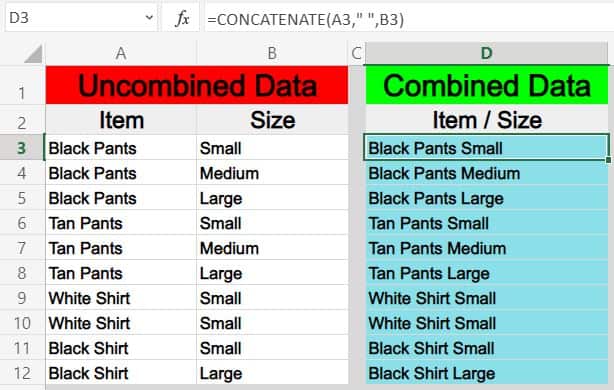
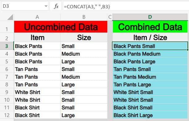
Notice that the CONCAT function (Shown Below) does the same thing as the CONCATENATE function (Shown Above)

=CONCAT(A3," ",B3)

Combine columns in Excel (Vertical)

Now I am going to show you how to combine columns in Excel vertically, or in other words "stack columns".

There are 2 different ways to combine columns in Excel vertically by using formulas, depending on how you would like the formula to operate:

• The first method (using the INDIRECT, ROW, and COUNTIF functions), will stack the column ranges that are specified on top of each other exactly as is
• The second method (using the INDEX, ROW, and MOD functions with an array), will combine the contents from individual columns into a single column, but will alternate between columns for each row

Formula for combining (stacking) columns in Excel:

=IF(A3<>"",A3,INDIRECT("B"&ROW()-COUNTIF(A$3:A$99,"<>")))

Formula for combining columns, while alternating back and forth between columns in Excel:

=INDEX($A$2:$B$99,ROW()/2,MOD(ROW(),2)+1)

* Note that both of these formulas must be copied / filled into the cells for the entire column (With one formula per cell).

Combining columns vertically while stacking one column on top of another column

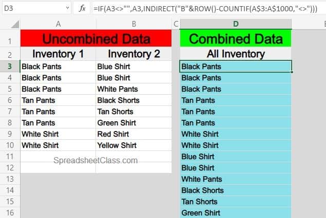
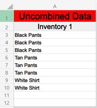
In this example we have two different lists of inventory that we want to combine into one. Let's say that two different employees counted clothing items in separate parts of your store, and that you want to combine the lists that they return to you into one list/column.

By using the INDIRECT function, the ROW function, and the COUNTIF function, we can create a formula that will stack the contents from one column, on top of the contents of another column. With the example / formula shown below, the contents of one entire column will be listed with the formula, before the contents of the second column are listed below it (As opposed to the alternating column method in the next example).

The task: Combine two lists of clothing items into a single list of unique inventory items… or in other words, make a single list that shows one of each item that is contained in inventory, by combining two lists

The logic: Combine the range A3:A10 and the range B3:B10 vertically into a single column

The formula: The formula below, is entered in the blue cell (D3), for this example

=IF(A3<>"",A3,INDIRECT("B"&ROW()-COUNTIF(A$3:A$1000,"<>")))

Make sure that you place your formula in the correct row, according to the beginning rows of the references in the formula (If the formula's references begin at row 3, make sure that your first formula is in row 3.

Note in the example image how the formula in cell D3 has been copied into the cells below it. Remember to do this in your sheet as well.

Combining columns vertically while alternating from column to column for each row

In this example we are going to combine the same inventory lists from the previous example, vertically into a single column, but this time we are going to use a different formula that alternates between columns when listing the combined column data (As opposed to stacking one entire column on top of another entire column).

To do this we will use the INDEX function, the ROW function, and the MOD function.

The task: Combine two lists of clothing items into a single list, and show all items found

The logic: Combine the contents in range A3:A10 and the contents in range B3:B10 vertically into a single column

The formula: The formula below, is entered in the blue cell (D3), for this example

=INDEX($A$2:$B$1000,ROW()/2,MOD(ROW(),2)+1)

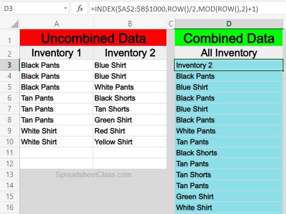
Like the formula in the previous example, make sure that your formula is placed in the correct row, according to the beginning rows of your formula references. However, with this particular formula, if your data begins on an odd row, such as row 3, your formula reference will need to begin on the previous / even row to make sure that all of the data is captured (As shown in the example image).

Note in the example image how the formula in cell D3 was copied into the cells below. Remember to do this in your sheet as well.

How to combine columns from separate sheets

You may find situations that require you to combine columns that are from separate tabs in Excel.

This can be done by simply referring to a certain tab name when specifying the ranges in the formula. So where you would normally set a range like "A1:C", when referencing another sheet while combining columns you will specify the tab name, by adding the tab name and an exclamation mark before listing the column and row for the range, like "TabName!A1:C"

However when the tab name has a space in it, you will need to use an apostrophe before and after typing the tab name, like 'Tab Name'!A1:C.

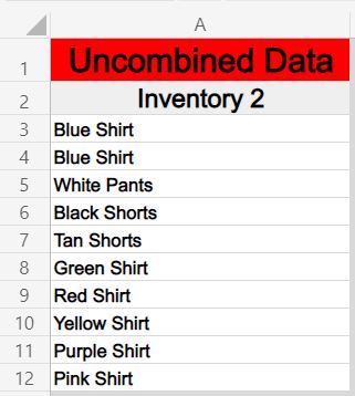
Here is an example of how to combine columns from multiple tabs in Excel, where there are two lists in different tabs, to be combined into a single list on a completely separate tab.

Let's say that you have a list of clothing items on one tab, another list of clothing items on a separate tab, and that you want to display a combined list of unique clothing items that are in inventory, on a completely different tab (meaning that there will be no duplicates).

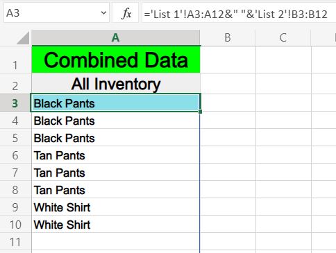
*Note that you can reference specified tabs with any of the formulas that you learned in this article, but for this example we are using an array with the ampersand (&) to demonstrate how to combine columns from different tabs.

The task: Combine the list of clothing items on the tab labeled "List 1", with the list of clothing items on the tab labeled "List 2" and show a combined list of clothing items, on completely separate tab

The logic: Combine the range 'List 1'!A3:A12, with the range 'List 2'!A3:A12

The formula: The formula below, is entered in the blue cell (A3), for this example

='List 1′!A3:A12&" "&'List 2′!B3:B12

Here are two different lists of clothing items, which are held on two separate tabs labeled, "List 1" and "List 2"

And here is a combined list of clothing items, where the formula and combined data are held on a separate tab

Pop Quiz: Test your knowledge

Answer the questions below about combining columns in Excel to refine your knowledge! Scroll to the very bottom to find the answers to the quiz.

Horizontal column combination formulas

=A3:A12&" "&B3:B12

=CONCAT(A3," ",B3)

=CONCATENATE(A3:A12," ",B3:B12)

Vertical column combination formulas

=IF(A3<>"",A3,INDIRECT("B"&ROW()-COUNTIF(A$3:A$1000,"<>")))

=INDEX($A$2:$B$1000,ROW()/2,MOD(ROW(),2)+1)

Question #1

Which of the following formulas will allow you to combine columns vertically? (Select all that apply)

1. =A3:A100&" "&B3:B100
2. =CONCAT(A5," ",B5)
3. =IF(A5<>"",A5,INDIRECT("B"&ROW()-COUNTIF(A$5:A$1000,"<>")))
4. =CONCATENATE(A3:A100," ",B3:B100)
5. =INDEX($A$5:$B$1000,ROW()/2,MOD(ROW(),2)+1)

Question #2

Which of the following formulas will put a space between the contents that are horizontally combined?

1. =CONCATENATE(A3:A100,B3:B100)
2. =A3:A100&" "&B3:B100

Question #3

True or False: For older versions of Excel, you must hold Ctrl + Shift + Enter on the keyboard before entering an array formula

1. True
2. False

Question #4

Which of the following formulas will combine columns horizontally?

1. =IF(A5<>"",A5,INDIRECT("B"&ROW()-COUNTIF(A$5:A$1000,"<>")))
2. =CONCATENATE(A3:A100," ",B3:B100)

Question #5

Which of the following formulas will stack / combine columns WITHOUT alternating between columns

• =IF(A5<>"",A5,INDIRECT("B"&ROW()-COUNTIF(A$5:A$1000,"<>")))
• =INDEX($A$5:$B$1000,ROW()/2,MOD(ROW(),2)+1)

---

Answers to the questions above:

Question 1: 3, 5

Question 2: 2

Question 3: 1

Question 4: 2

Question 5: 1