

There are a variety of different ways to combine columns in Google Sheets, and I am going to show you six different formulas that you can use to combine multiple columns into one. Three of these formulas will combine columns horizontally, and three of them will combine columns vertically.
Directly below are quick instructions for combining columns, but also look further below for detailed examples, as well as additional ways of combining columns.
This lesson also includes how to combine more than 2 columns, as well as how to filter out blanks spaces from your combined columns.
To combine columns horizontally in Google Sheets, follow these steps:
- Type =ARRAYFORMULA( to begin your formula for combining columns
- Type the address for the first column that you want to combine with, such as A1:A
- Type an ampersand (&)
- Type the address of the other column that you want to combine with, such as B1:B
- Press enter on the keyboard. The full formula will look like this: =ARRAYFORMULA(A1:A&B1:B)
To combine columns vertically in Google Sheets, follow these steps:
(See detailed instructions below for how to add spaces or special characters between the columns)
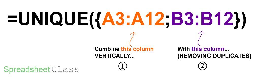
- Type =UNIQUE({ to begin your formulas / array
- Type the address for the first column that you want to combine with, such as A1:A
- Type a semicolon (;)
- Type the address of the other column that you want to combine with, such as B1:B
- Type a closing curly bracket ( } )
- Press enter on the keyboard. The full formula will look like this: =UNIQUE({A1:A;B1:B})
Here are the formulas that will combine columns in Google Sheets:
Horizontal column combination formulas
- =ARRAYFORMULA(A3:A&” “&B3:B)
- =ARRAYFORMULA(CONCAT (A3:A,B3:B))
- =JOIN(” “,A3,B3)
Vertical column combination formulas
- ={A3:A12;B3:B12}
- =UNIQUE({A3:A12;B3:B12})
- =FILTER({A3:A12;B3:B12}, LEN({A3:A12;B3:B12}))
Download your column combining cheat sheet
Click here to get your Google Sheets cheat sheet
This lesson will teach you how to combine columns in Google Sheets, but check out this article if you want to learn how to combine columns in Excel.
Combine columns in Google Sheets (Horizontal)
First I am going to show you how to combine columns in Google sheets horizontally.
If you have two columns that you would like to combine the contents of, where the values of the cells in each row are to be combined together horizontally, then there are a couple simple ways of doing this:
- The first method (using the ARRAYFORMULA function with the “&” operator / ampersand), will allow you to not only combine/merge two columns horizontally, but will also allow you to separate the contents with specified values/ strings of text, and will also allow you to combine more than two columns if you wish
- The second method (using the ARRAYFORMULA function with the CONCAT function), will allow you to combine the contents of two or more columns horizontally. The CONCATENATE function is almost identical to CONCAT, and I will mention more about this function below.
- The third method (using the JOIN function), will allow you to combine the contents of two or more cells / columns horizontally.
Each of these methods can be used to combine individual cells, without having to use the ARRAYFORMULA function.
Using ARRAYFORMULA / & (Ampersand) to combine columns
First I will show you the most common and functional way of combining columns horizontally in Google Sheets.
By using the ARRAYFORMULA function with the “&” operator you will be able to combine multiple columns in Google Sheets, and you will also be able to specify values and strings of text that you would like to attach to the column combination.
To combine the data from individual cells, follow these steps:
- Type an equals sign, and then type the address for the first cell that you want to combine with, such as A3
- Type an ampersand (&)
- Type the address of the another cell that you want to combine with, such as B3
- Press enter on the keyboard. The full formula will look like this: =A3&B3
- Copy / fill down the formula to use it on the entire column, or apply the ARRAYFORMULA function
Here is more information on using the ARRAYFORMULA function, as well as copying formulas.
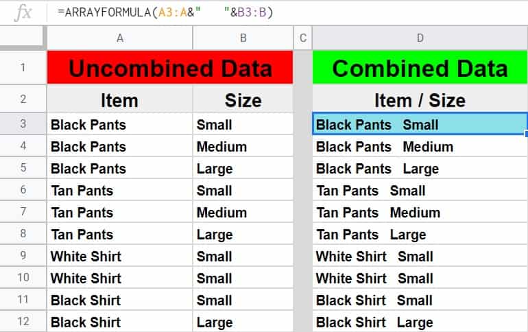
In this first example we have a list of clothing inventory items in one column, and the clothing size for that item listed in another column… and we want to combine these columns horizontally so that in each row the clothing item and size are displayed as a single text string, in a single column.
We will also put a separating space between the contents that are combined in this example. This is accomplished by using quotation marks with a space between them i.e. (” “) in the array formula (shown below).
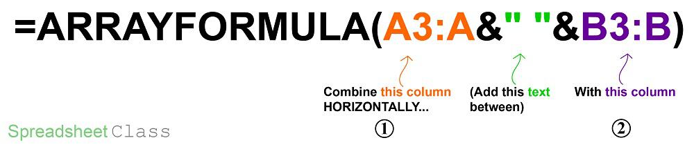
The task: Horizontally combine the “item” column with the “size” column, and put a space between the contents… so that the clothing item and size are displayed in a single column.
(Where the contents of the cells in each row are combined into a single text string separated by a space)
The logic: Horizontally combine the contents of the cells in the range A3:A, with the contents of the cells from the range B3:B, and add a space between the text/contents from the combined columns
The formula: The formula below, is entered in the blue cell (D3), for this example
=ARRAYFORMULA(A3:A&” “&B3:B)
(Note: The ARRAYFORMULA function shown above is also perfect for combining first and last name!)
Combining more than 2 columns horizontally
If you want to combine more than 2 columns horizontally in Google Sheets, you can do this with the ARRAYFORMULA function and the “&” operator, which is also called an “ampersand”.
For example, if you wanted to combine columns A, B and C, horizontally (with spaces between), then you could use the formula below.
=ARRAYFORMULA(A3:A&” “&B3:B&” “&C3:C)
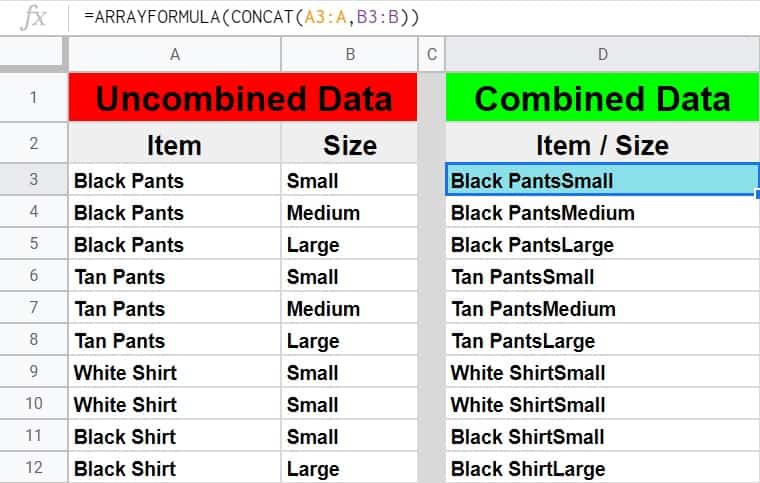
Using ARRAYFORMULA / CONCAT to merge columns in Google Sheets
In this example we want to achieve the same task as in the first example (merge the “item” column with the “size” column horizontally), however we are going to use a different formula.
We will be using the CONCAT function, which is compatible with the ARRAYFORMULA, making it easy to combine an entire column with a single formula.
However, note that you can also use the CONCATENATE function to combine cells and even place spaces / characters between those columns, just like we did with the “&” symbol… but the CONCATENATE function does not work with the ARRAYFORMULA function, and so if you use this to combine columns you will need to use one formula in each cell.
To combine the data from cells with the CONCAT formula, follow these steps:
- Type =CONCAT ( to begin your formula
- Type the address of the first cell that you want to combine with, such as A2
- Type a comma, and then type the address of the next cell that you want to combine with, such as B2
- Press enter on the keyboard. The full formula will look like this: =CONCAT (A3,B3)
- Copy / fill down the formula to use it on the entire column, or apply the ARRAYFORMULA function
To combine the data from cells by using the CONCATENATE, follow these steps:
- Type =CONCATENATE ( to begin your formula
- Type the address of the first cell that you want to combine with, such as A5
- Type a comma, and then type the address of the next cell that you want to combine with, such as B5
- Press enter on the keyboard. The full formula will look like this: =CONCATENATE (A5,B5)
- Copy / fill down the formula to use it on the entire column
See the example / instructions above for how to add spaces / special characters between the columns. Again if you want to learn more about expanding formulas, check out these articles on using the ARRAYFORMULA function, as well as copying / filling formulas.
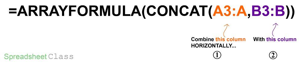
The task: Horizontally combine the column that shows clothing items with the column that shows clothing sizes… so that the clothing item and size are displayed in a single column.
(Where the contents of the cells in each row are combined into a single text string)
The logic: Combine the range A3:B, and the range B3:B into a single column, so that the contents from the cells are horizontally merged into a single text string
The formula: The formula below, is entered in the blue cell (D3), for this example
=ARRAYFORMULA(CONCAT (A3:A,B3:B))
Using the JOIN function to combine cells / columns in Google Sheets
Another formula that can be used to combine cells, or combine columns, is the JOIN function. The JOIN function, like the CONCATENATE function, cannot be used with the ARRAYFORMULA function (must be used with one formula for each row), so in this example I’ll briefly go over how to copy and paste / autofill a formula down the column, but check out the linked article for more detail.
The JOIN function is different than the CONCATENATE function because you can specify the “delimiter” or in other words you can specify what character(s) you want to separate the combined / concatenated cells.
Syntax:
JOIN(delimiter, value_or_array1, [value_or_array2, …])Formula summary: “Concatenates the elements of one or more one-dimensional arrays using a specified delimiter.”
So to use the JOIN function, first you specify what character(s) / number(s) etc. (if any) that you want to separate the combined data, type a comma, then specify the first cell, type a comma, and then specify the second cell to combine the first with.
The task: Horizontally combine the column that shows clothing items with the column that shows clothing sizes… so that the clothing item and size are displayed in a single column.
(Where the contents of the cells in each row are combined into a single text string)
The logic: Combine the range A3:B, and the range B3:B into a single column, so that the contents from the cells are horizontally merged into a single text string
The formula: The formula below, is entered in the blue cells. It is initially into the cell D3, and then copied/filled into the range D3:D12
=JOIN(” “,A3,B3)
This example used a space between the combined data, but if you do not want a space, your formula would look like this: =JOIN(,A3,B3)
Or if you want to include a word between the combined data, your formula would look like this: =JOIN(“Text”,A3,B3)
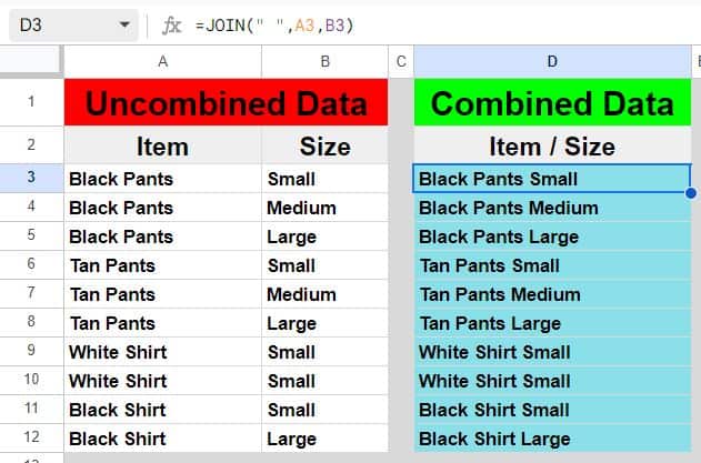
As you can see in the image above, the data from column A has been horizontally combined with the data from column B, with a space put in between.
After entering the first formula to combine the first row of cells, then we can simply copy and paste cell D3 into the cells below, and Google Sheets will automatically put the correct formula with the correct references in each cell, allowing you to combine the data from the columns horizontally, as far down as you copy and paste the formulas.
You can also use “Autofill” to do the same thing, by hovering your cursor on the bottom right of the cell with a formula in it, until the plus sign / crosshairs appears, click your mouse, hold the click, and drag your cursor downwards until you have reached the row where you want to copy the formula to, and release the click. See the articles linked above for a detailed lesson on this.
Combine columns in Google Sheets (Vertical)
Now I am going to show you how to combine columns in Google Sheets vertically, or in other words “stack columns”.
There are 3 different ways to combine columns in Google Sheets vertically by using formulas, depending on how you would like the formula to operate:
- The first method (using an array with a semicolon separator), will stack the column ranges that are specified on top of each other exactly as is, including duplicates and empty spaces
- The second method (using the UNIQUE function with an array), will stack the column ranges that are specified on top of each other… while removing duplicates
- The third method (using the FILTER function with the LEN function), will stack the column ranges that are specified on top of each other… while removing spaces but keeping duplicates
Using arrays in Google Sheets
In some Google Sheets formulas, you will need to use what is called an “array”. An array is similar to what the ARRAYFORMULA does, but it is notated by using curly brackets { } (i.e. braces). In the example below you will see curly brackets used to create arrays. Make sure to include the curly brackets in your formula so that they work properly.
Using an array with a semicolon separator to combine columns
In this example we have two different lists of inventory that we want to combine into one. Let’s say that two different employees counted clothing items in separate parts of your store, and that you want to combine the lists that they return to you into one list/column.
By using an array of two different ranges separated by a semicolon, you can stack the contents of those ranges on top of each other exactly as is, meaning that the resulting range/column will retain any spaces and duplicates that are contained in the specified ranges to be combined.
(If you use a comma instead of a semicolon, it will combine the range horizontally instead of vertically). Later I will show you how to filter out blank spaces if you want.
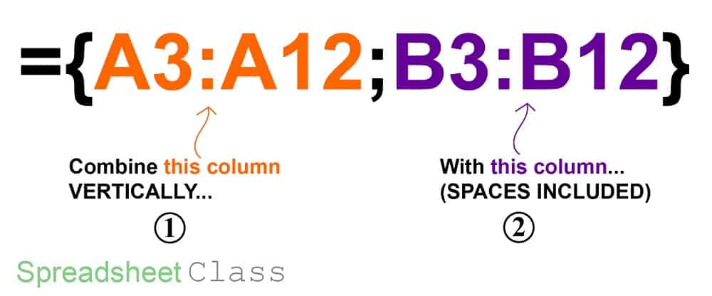
The task: Combine the individual clothing inventory lists vertically into one long inventory list
The logic: Combine the range A3:A12 and the range B3:B12 vertically into a single column, including any spaces or duplicates
The formula: The formula below, is entered in the blue cell (D3), for this example
={A3:A12;B3:B12}

Combining more than 2 columns vertically with an array
If you want to combine more than 2 columns vertically in Google Sheets, you can do this with an array separated by a semicolon, just like in the previous example, but you can keep adding semicolons and ranges if you wish.
For example if you wanted to stack/combine columns A, B, C, and D vertically, then you could use the formula below.
Remember that this method will keep duplicates, and any empty spaces that are within the source ranges. But in the next example I’ll show you how to filter out blank spaces.
The task: Combine columns A through D into a single column
The logic: Combine the ranges A3:A9, B3:B9, C3:C9, and D3:D9, vertically into a single column, including any spaces or duplicates
The formula: The formula below, is entered in the blue cell (F3), for this example
={A3:A9;B3:B9;C3:C9;D3:D9}
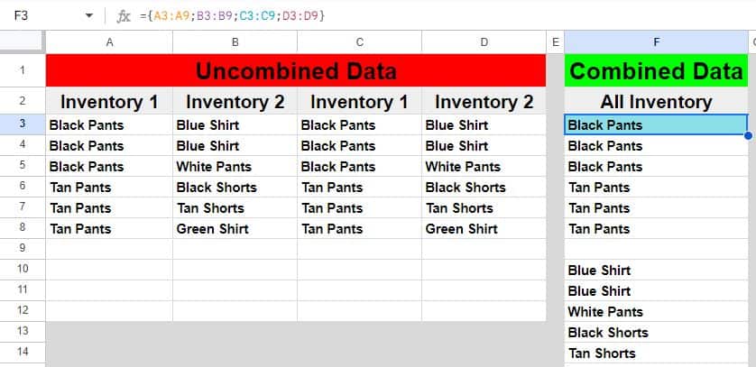
As you can see in the image above, the data from columns A through D is now combined into a single column of data, in column F.
Note that this same method of using additional semicolons and ranges to combine more and more columns, can be used at the same time as using the UNIQUE formula as described in a later example.
How to filter out blank spaces when combining columns
Okay now let’s go over how to filter out the blank spaces from your combined columns. We will do this by using the FILTER formula.
The task: Combine columns A through D into a single column
The logic: Combine the ranges A3:A9, B3:B9, C3:C9, and D3:D9, vertically into a single column, and filter out the blank spaces
The formula: The formula below, is entered in the blue cell (F3), for this example
=filter({A3:A9;B3:B9;C3:C9;D3:D9},{A3:A9;B3:B9;C3:C9;D3:D9}<>””)
This formula tells Google Sheets to filter the combined range / data, and only display the rows that are not blank.
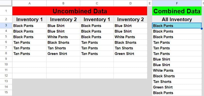
As you can see in the image above, the data from columns A through D has been combined into a single column, but the blank spaces have been filtered out.
Using UNIQUE with an array to combine columns and remove duplicates
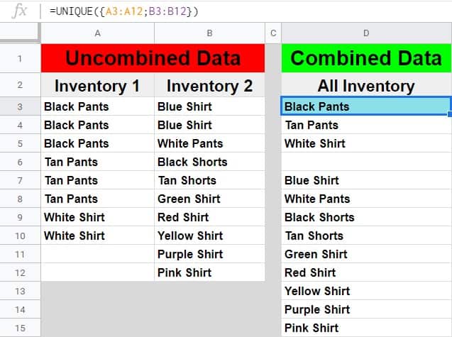
In this example we also have two lists of clothing items found in inventory, and we also want to combine them vertically into a single column… but this time we want to remove any duplicates, and generate a list of unique inventory items (one of each).
By using the same method from the previous example (an array separated by a semicolon), with the UNIQUE function wrapped around it, the list of values that is created will not contain duplicates… and for that same reason the list will only contain up to one empty space in the results.
(In the next example I’ll show you how to remove spaces without removing duplicates)
The task: Combine two lists of clothing items into a single list of unique inventory items… or in other words, make a single list that shows one of each item that is contained in inventory, by combining two lists
The logic: Combine the range A3:A12 and the range B3:B12 vertically into a single column, removing any duplicates
The formula: The formula below, is entered in the blue cell (D3), for this example
=UNIQUE({A3:A12;B3:B12})
Combining more than 2 columns vertically with a unique array
If you want to combine more than 2 columns vertically in Google Sheets, while removing duplicates, you can do this with an array wrapped in the UNIQUE function. As described in an earlier example, to add another range to combine / stack, simply add another semicolon and another range to combine into the single column.
For example if you wanted to stack/combine columns A, B, and C vertically, and to remove any duplicates found in the source range, you could use the formula below.
=UNIQUE({A3:A9;B3:B9;C3:C9;D3:D9})
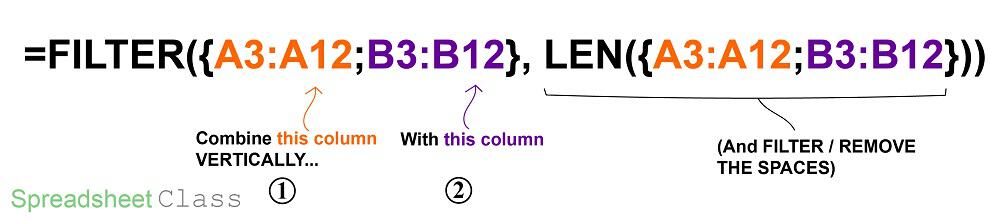
Using FILTER with LEN to combine columns and remove spaces
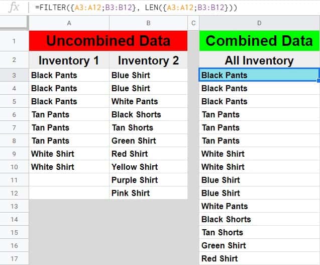
In this example we are going to combine the same inventory lists from the previous example, vertically into a single column, but this time we are going to keep any duplicates and remove any empty spaces.
To do this we will create a stacked array as in the previous example, but we will use the FILTER function with the LEN function to remove / filter out empty spaces.
The task: Combine two lists of clothing items into a single list, and show all items found, without no empty spaces
The logic: Combine the contents in range A3:A12 and the contents in range B3:B12 vertically into a single column, and filter out any empty spaces
The formula: The formula below, is entered in the blue cell (D3), for this example
=FILTER({A3:A12;B3:B12}, LEN({A3:A12;B3:B12}))
Combining more than 2 columns vertically with FILTER / LEN
If you want to combine more than 2 columns vertically in Google Sheets, while keeping duplicates but removing any empty spaces, you can do this with the FILTER function and the LEN function.
For example if you wanted to stack/combine columns A, B, and C vertically, and to keep duplicates but remove empty spaces found in the source range, you could use the formula below.
=FILTER({A3:A12;B3:B12;C3:C12}, LEN({A3:A12;B3:B12;C3:C12}))
How to combine columns from separate sheets
You may find situations that require you to combine columns that are from separate tabs in Google Sheets.
This can be done by simply referring to a certain tab name when specifying the ranges in the formula. So where you would normally set a range like “A1:C”, when referencing another sheet while combining columns you will specify the tab name, by adding the tab name and an exclamation mark before listing the column and row for the range, like “TabName!A1:C”
However when the tab name has a space in it, you will need to use an apostrophe before and after typing the tab name, like ‘Tab Name’!A1:C.
Here is an example of how to combine columns from multiple tabs in Google Sheets, where there are two lists in different tabs, to be combined into a single list on a completely separate tab.
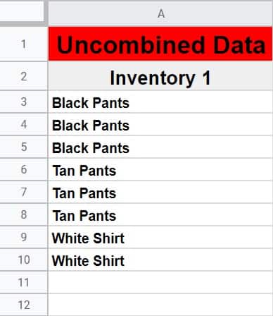
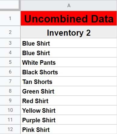
Let’s say that you have a list of clothing items on one tab, another list of clothing items on a separate tab, and that you want to display a combined list of unique clothing items that are in inventory, on a completely different tab (meaning that there will be no duplicates).
*Note that you can reference specified tabs with any of the formulas that you learned in this article, but for this example we are using a unique array to demonstrate how to combine columns from different tabs.
The task: Combine the list of clothing items on the tab labeled “List 1”, with the list of clothing items on the tab labeled “List 2” and show a combined list of clothing items (without duplicates), on completely separate tab
The logic: Combine the range ‘List 1’!A3:A12, with the range ‘List 2’!A3:A12, removing any duplicates
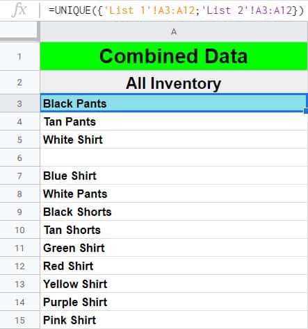
The formula: The formula below, is entered in the blue cell (A3), for this example
=UNIQUE({‘List 1′!A3:A12;’List 2’!A3:A12})
Here are two different lists of clothing items, which are held on two separate tabs labeled, “List 1” and “List 2”
And here is a combined list of clothing items, where the formula and combined data are held on a separate tab
Use “Split text to columns” to split text into columns and back again
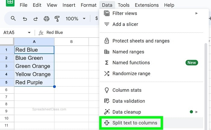
Sometimes you may want to split text into columns, and the easiest way to do this is to use “Split text to columns”, as shown in the image below. Select the data to split, then click “Data”, and then click “Split text to columns”. Then choose the appropriate separator (such as “Space” or “Comma”), and the text will be split into individual columns.
Then while the range is still selected, you can choose another separator to combine the text into one column again.
How I combine columns in my work
Horizontally: The most common way that I use these formulas to combine columns horizontally at my job, is to combine first and last names for students, and to make unique identifiers. Student data usually comes with first and last names listed in separate columns, but for the dashboards that I build I like to have the full name in “Last, First” format in a single column.
I also use these formulas to make unique identifiers, such as when a report does not contain an ID number and I need to combine a student name with another piece of information to ensure that I can call upon a unique ID to use XLOOKUP (since some students have the exact same first and last name and using their name alone as the “ID” causes the wrong data to be pulled in for duplicate names.
Vertically: The most common way that I use these formulas to combine columns vertically in my work, is when I need to combine several reports that are in the same format, but exported separately. For example one of the online curriculum platforms that students work in export their data one grade level at a time, and for the dashboard I have to combine the reports together into one vertically stacked comprehensive report.
Pop Quiz: Test your knowledge
Answer the questions below about combining columns in Google Sheets to refine your knowledge! Scroll to the very bottom to find the answers to the quiz.
Classroom downloads:
Combining columns cheat sheet (PDF)
Click here to get your Google Sheets cheat sheet
Or click here to take the dashboards course
Click the green “Print” button below to print this entire article.
Question #1
Which of the following formulas will allow you to combine columns vertically? (Choose all that apply)
- =ARRAYFORMULA(A1:A&” “&B1:B)
- ={C3:C12;D3:D12}
- =FILTER({A7:A14;B7:B14}, LEN({A7:A14;B7:B14}))
- =ARRAYFORMULA(CONCAT (A5:A,B5:B))
- =UNIQUE({A1:A11;B1:B11})
Question #2
Which of the following formulas will put a space between the contents that are horizontally combined?
- =ARRAYFORMULA(CONCAT (F3:F,G3:G))
- =ARRAYFORMULA(G4:G&” “&H4:H
Question #3
True or False: The following formula will remove all duplicates and empty spaces when combining columns: ={Y1:Y2;Z1:Z2}
- True
- False
Question #4
Which of the following formulas will remove duplicates from the combined column?
- =FILTER({A17:A100;B17:B100}, LEN({A17:A100;B17:B100}))
- =UNIQUE({C5:C15;D5:D15})
- ={A2:A20;B2:B20}
Question #5
Which of the following formulas will remove empty spaces from the combined column, but not duplicates?
- =FILTER({K3:K12;L3:L12}, LEN({K3:K12;L3:L12}))
- =UNIQUE({V3:V12;Z3:Z12})
- ={J2:J12;U2:U12}
Answers to the questions above:
Question 1: 2, 3, 5
Question 2: 2
Question 3: 2
Question 4: 2
Question 5: 1