

In this lesson I am going to teach you how to create drop-down lists in Google Sheets. Creating a drop-down list is done by something that is called “Data Validation”. Drop-down lists are extremely useful, and they assure that only valid data is entered into the cells. Drop-downs also make it very easy and fast to select the correct text / enter data into cells.
When I was a data integration specialist, I used drop-down menus frequently for two main purposes: #1 To make it simple for staff members to select the exact selections / text in manual spreadsheet trackers, so that I could have accurate data without people misspelling words… and #2 to create interactive dashboards and reports, such as creating a custom drop-down that allows people to filter data / a chart how they want.
But of course there are many more things that you can do with drop-down menus.
(Google Sheets recently updated the menus for data validation, and this lesson is also updated to demonstrate the current menus / methods).
To create a drop-down list in Google Sheets, follow these steps:
- Select the cell / range of cells that you want to create a drop-down list in
- On the top toolbar, click “Data” (A menu will appear)
- Click “Data validation” (Another menu will appear)
- Click “Add rule”, and a menu will pop up on the right
- Under the “Criteria” selection, choose between “Dropdown”, or “Dropdown (from a range)”
- If you choose, “Dropdown”, list the items for your drop-down list in the blank fields below the “Criteria” menu
- If you choose “Dropdown (from a range)”, type / select the range of cells that contains your criteria list, then press “Enter” on the keyboard, and Google Sheets will automatically list the items within that range, in the blank fields below the “Criteria” menu
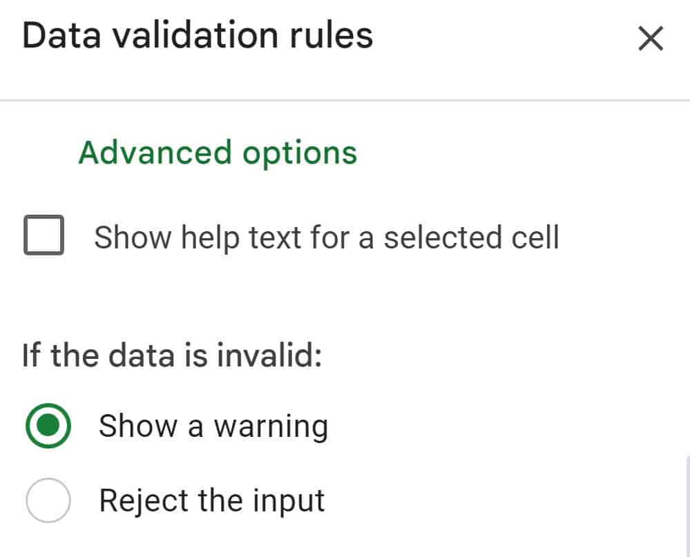
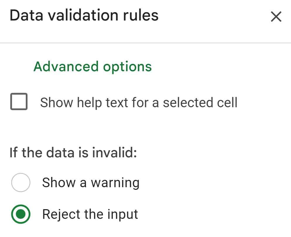
- (Optional): Click “Advanced options” and choose between “Show a warning”, or “Reject the input” (Default is set to “Reject the input)
- Click “Done”. A drop-down will now be present in the cell that you selected
Below I will go over several examples of creating a drop-down and applying data validation in Google Sheets. I will go over the various ways to create the drop-down, how to copy the drop-downs to other cells, and what different settings in the data validation menu will do.
Note that you can delete the contents of a cell that has a drop-down menu in it by pressing delete or backspace on the keyboard, and your drop-down list / data validation will still be present, but if you press the “Delete” button while the cell is empty, the dropdown menu will be removed from the cell. See more below about removing data validation from cells.
Check out the “interactive dashboard” tutorial in my full dashboards course to see how drop-down lists can be used to filter data based on the selection, update cell values based on the selection, and to make an entire chart / dashboard interactive.
List of items vs. List from range
When creating a drop-down list, you will have the option to base your drop-down list on a list of items, or you can choose to list from a range.
When you choose “Dropdown” from the criteria menu (in the data validation menu), you will type your list of dropdown items directly into the data validation menu. To edit the list, you will need to visit the data validation menu each time.
If you choose “Dropdown (from a range) you will type the items in the list into cells in your spreadsheet, and then you will type the range / cell address that contains the list. With this method, you can modify your list by editing the contents of the spreadsheet cells.
Applying drop-down lists to multiple cells at once
If you select a range of cells instead of a single cell before opening the data validation menu (or if you type the address of a range of cells in the “Apply to range” field), the data validation settings / drop-down lists will be applied to the entire range of selected cells. You can also copy and paste drop-downs from one cell into other cells, which I will show you later.
How to create a drop-down list in Google Sheets
First let’s go over an example of creating a drop-down list in Google Sheets, based on a list of items.
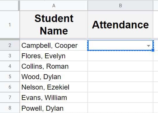
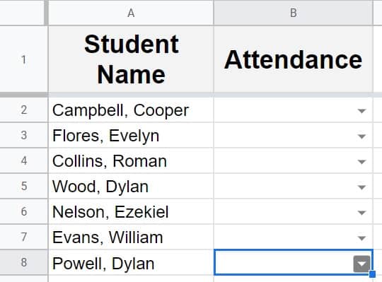
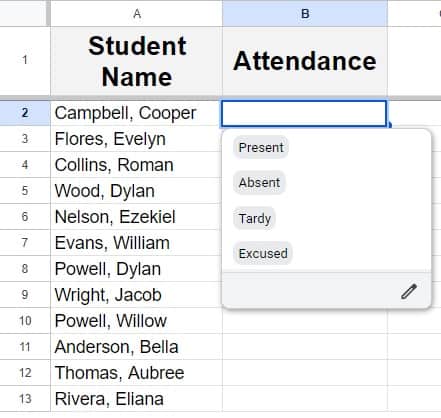
Below we have an example that shows a list of students, and an empty column beside it, where we want to create a drop-down list to enable selecting each student’s attendance status. We will make a simple drop-down list that allows the user to select between two choices (Present, and Absent). Follow the instructions below to learn how to do this.
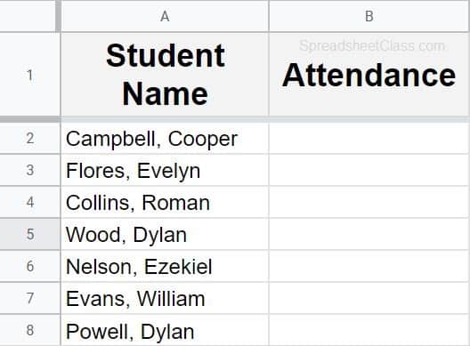
Select the cell / range of cells where you want your drop-down list to be. This example demonstrates creating a drop-down in cell B2.
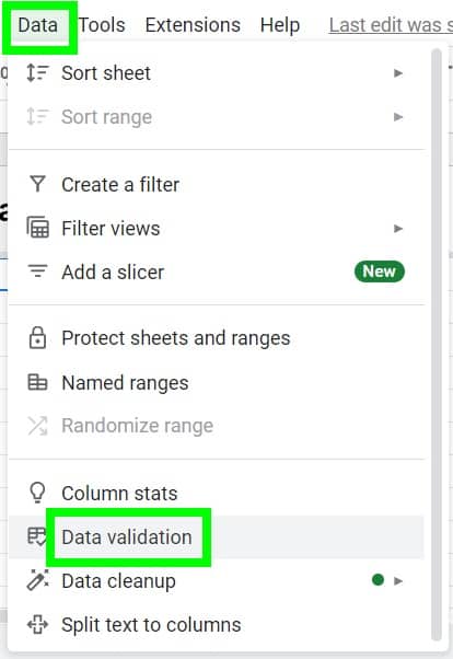
On the top toolbar menu, click “Data”. This will open a menu below. Then click “Data validation”. This will open the data validation menu, which is the place to create a drop-down list.
Side note: Another way to open the data validation menu, is to right-click on the cell, then click “View more cell actions”, and then click “Data validation”. You can also right-click on a cell and then click “Dropdown” which will create a dropdown menu and open the data validation menu.
Under the “Criteria” selection, select “Dropdown”. (You can also select “Dropdown (from a range)”, but this example demonstrates the “List of Items” option.
Notice in the “Apply to range” field, the cell range appears like this: Sheet1!B2. This could have been typed manually, but Google Sheets automatically filled it in because we selected the appropriate range before opening the menu.
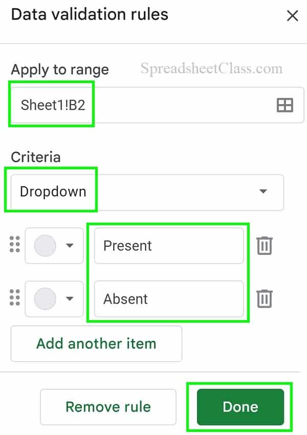
Type the items that you want in your drop-down list, in the blank fields below the “Criteria” menu. You can also select a custom color to the left of the listed item, if you wish.
Click “Advanced options”, and then choose between “Show a warning” or “Reject the input”. The default for this option is “Reject the input”.
Click “Done“.
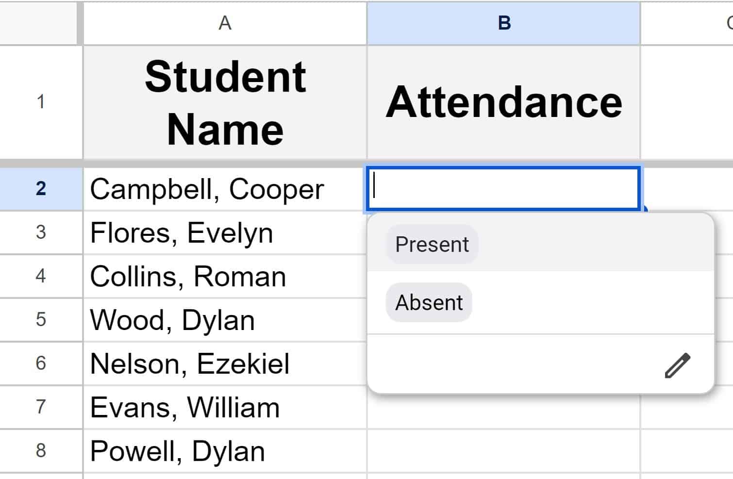
As shown below, after applying data validation, a triangular arrow appears inside of a small box, on the right side of the cell. This indicates that a drop-down list is present. If you hover your cursor over the small box with the arrow, the box will turn grey. If you click the arrow, the drop-down list / menu will open.
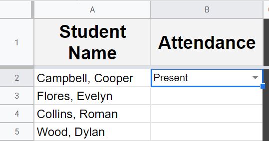
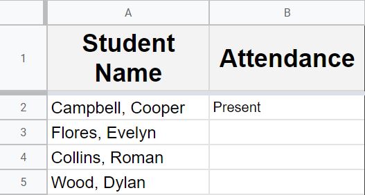
After clicking the drop-down button, the items that you typed in the data validation menu will appear in your drop-down list. When you click on one of the items in the list, Google Sheets will automatically fill the cell with the text / value that you selected.
Note that if you had selected the range B2:B8 before opening the data validation menu (Instead of only cell B2), the drop-down lists would have been applied to cells B2 through B8.
List from a range of cells to create a drop-down list
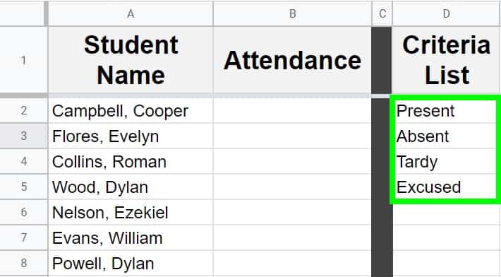
Now let’s go over an example where we will list the items for the drop-down list, in spreadsheet cells. We are using another example of student attendance, but this time we will add in a couple more items / selections to the list.
When you list your drop-down items in spreadsheet cells, it makes it very fast and easy to modify the list of items for your drop-down list. When you edit the list that is entered into the spreadsheet cells, the list in the drop-down will automatically reflect the change. This also allows you to use formulas that modify the list of items, which I will go over further below.
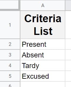
As you can see below, the items are entered into the range D2:D5. The following words are entered into cells D2 through D5: Present, Absent, Tardy, Excused. We are going to refer to this range of cells in the data validation menu, to base our drop-down list on the list of items in column D. To do this, follow the instructions below.
Select the cell / range of cells that you want to put drop-down lists in. This example demonstrates creating a drop-down in cell B2.
On the top toolbar, click “Data”, then click “Data Validation”.
Click “Add rule”
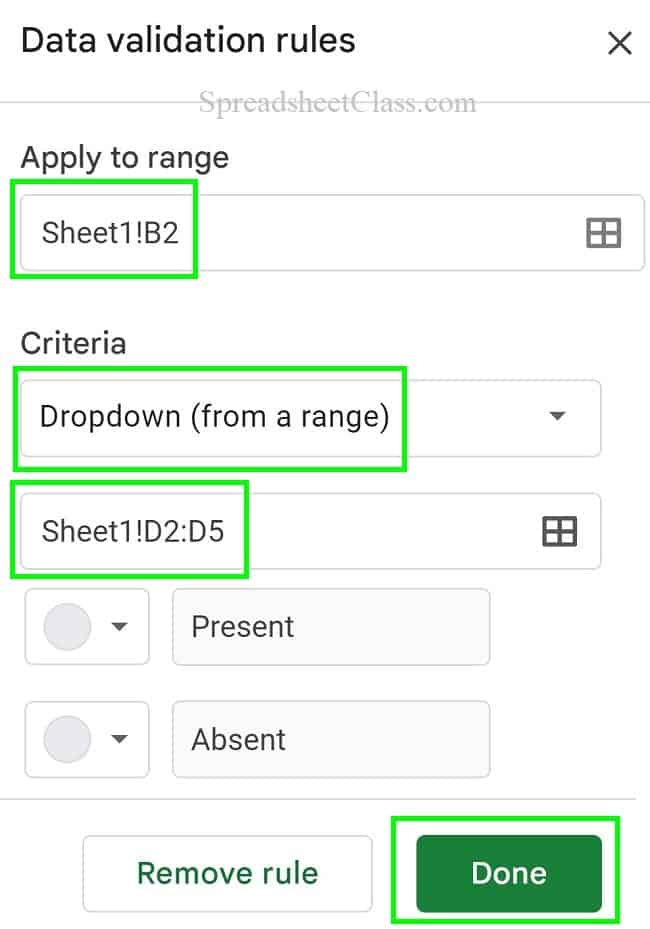
Under the “Criteria” option, select “Dropdown (from a range)”.
Type the range of cells that contains the list for your drop-down (Or you can use the “Select data range” button to specify the range without typing it manually. This button looks like a small grid). In this example we are typing the range D2:D5 (Google Sheets may automatically add the tab name to your reference, after you enter the range, such as “Sheet1!D2:D5”. No need to worry about this.)
Choose between “Show a warning”, or “Reject the input”, and then click “Done”.
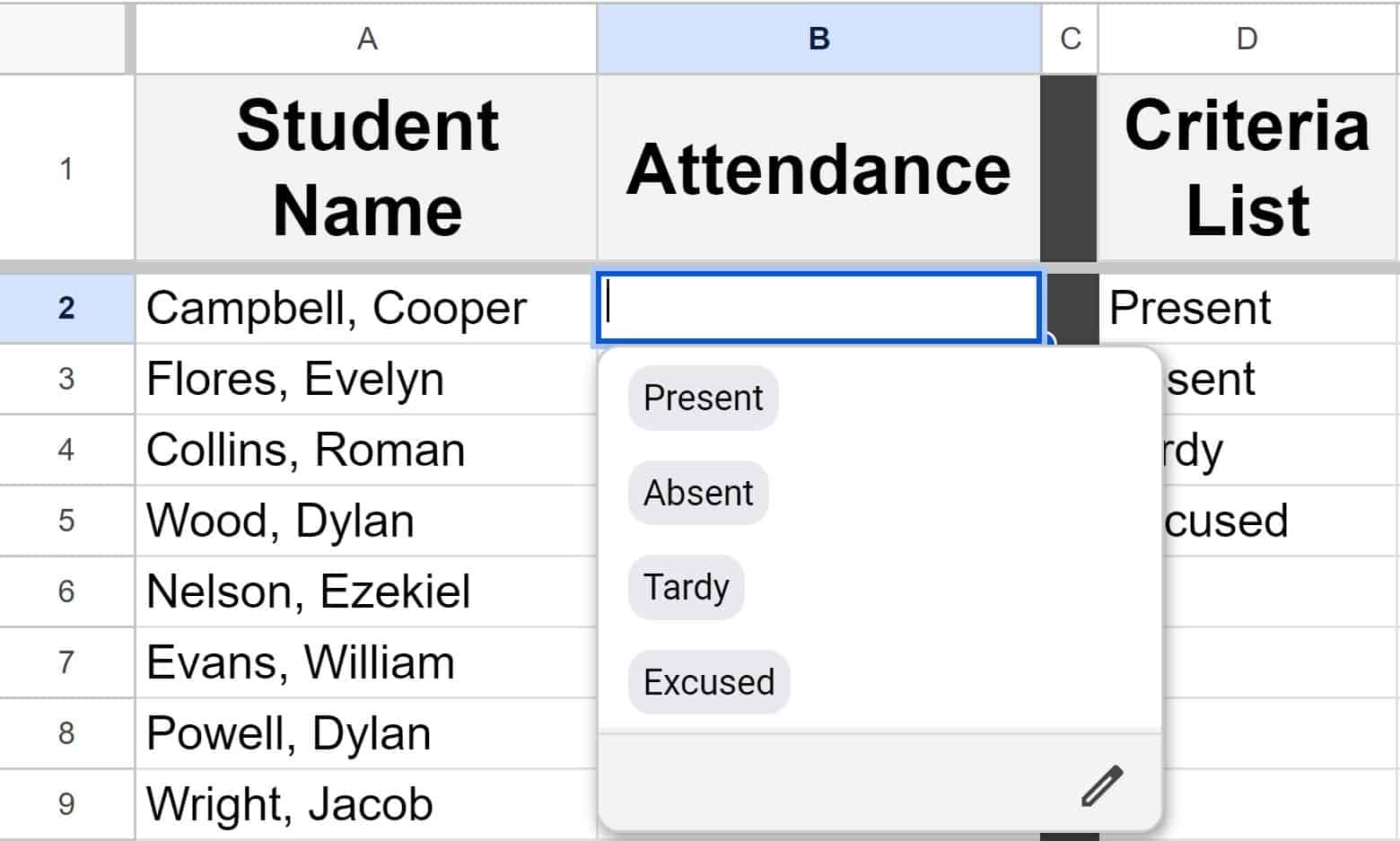
As shown below, after applying data validation to cell B2, with the “Dropdown (from a range)” field referring to the range D2:D5, a drop-down list has appeared in cell B2, and the items that are listed in column D are also listed in the possible selections for the drop-down menu.
Multiple ways to enter / select the range
There are two different ways to specify the cell / range of cells that you want the data validation to be applied to… or in other words the cells that you want the drop-down lists to be in. First, you can select the appropriate cell / range of cells before opening the data validation menu, as described in the examples in this lesson. When you do this, Google Sheets will automatically fill in the data range address. Or, you can type the cell address directly into the data validation menu, under the “Apply to range” field. For example, if the data validation is applied to cell B2 in the tab named “Sheet1”, then the cell range in the data validation menu will appear as Sheet1!B2
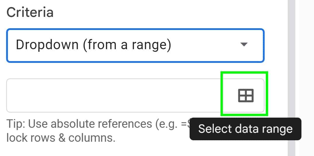
There are two different ways to specify the range that contains the list items for the “Dropdown (from a range)” option. First, you can type the address directly into the data validation menu, or as is shown below, you can use the “Select data range” button.
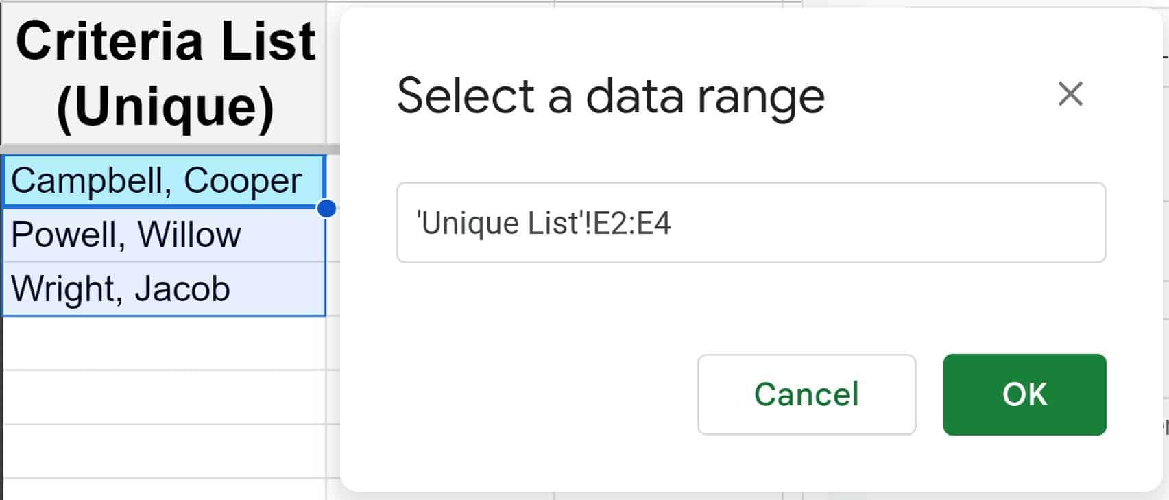
To select the data range instead of typing it, click the button that looks like a grid (Says “Select data range” when you hover your cursor over it). A small menu will pop up.
Then select the cell / range of cells that contains the items for the drop-down list. Then click “OK”.
Using the UNIQUE function to create a criteria list
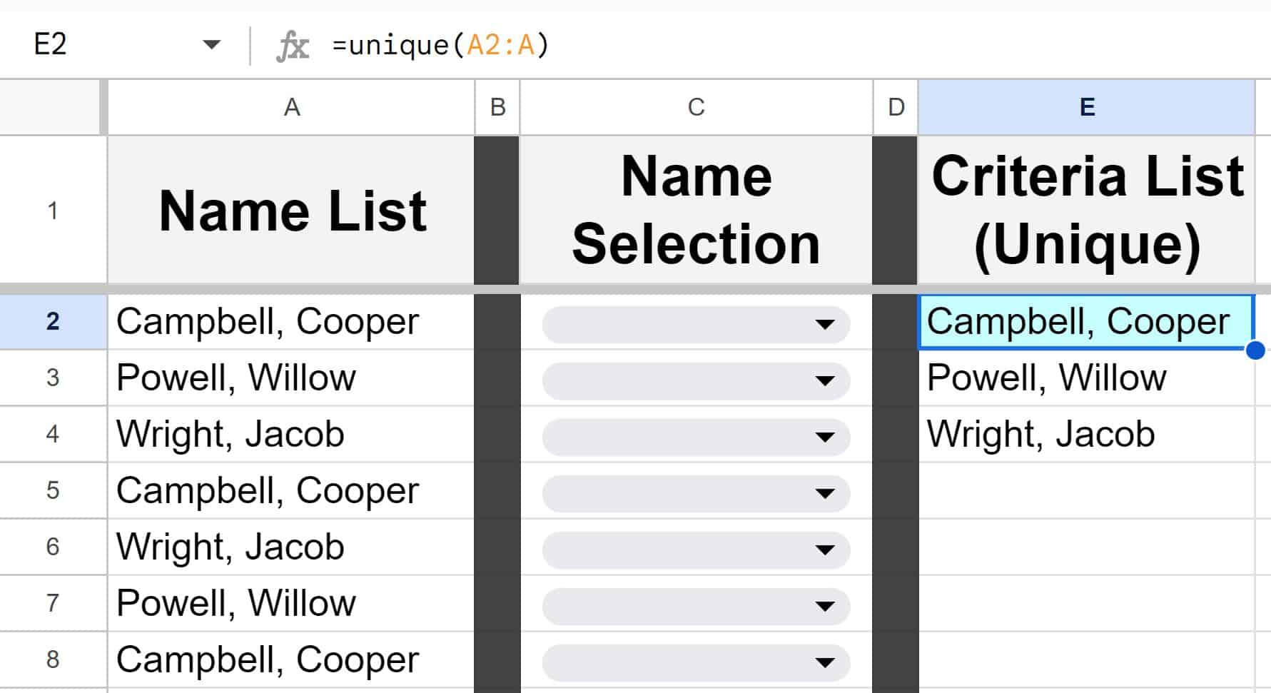
A great trick to use with drop-down lists in Google Sheets, is to use the UNIQUE function to generate a list of items for your drop-down menu, when there are duplicates present in the column that you are referring to. In the example below, you can see in column A that there are duplicate names. If we want to use this column to find a list of unique (non-duplicate) names so that we can refer to it with a drop-down list, we can simply use the UNIQUE function as shown below.
In cell E2, we are using the UNIQUE function to remove the duplicates from column A, which gives us a list of unique names in column E. We can then refer to column E in the data validation menu, to use the unique list of names as the drop-down list items.
Formula: =UNIQUE(A2:A)
Show a warning vs. Reject the input
You can choose how you want your spreadsheet to respond when someone enters invalid data into a cell with a drop-down / data validation.
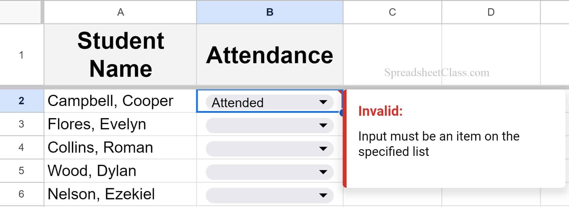
The first option is to “Show a warning” when invalid data is entered, which will display a warning in the cell (Small red triangle with a message that pops up when you hover over it). In the images below you can see where this option is selected in the data validation menu, as well as the warning that displays when invalid data is entered with the “Show warning” option.
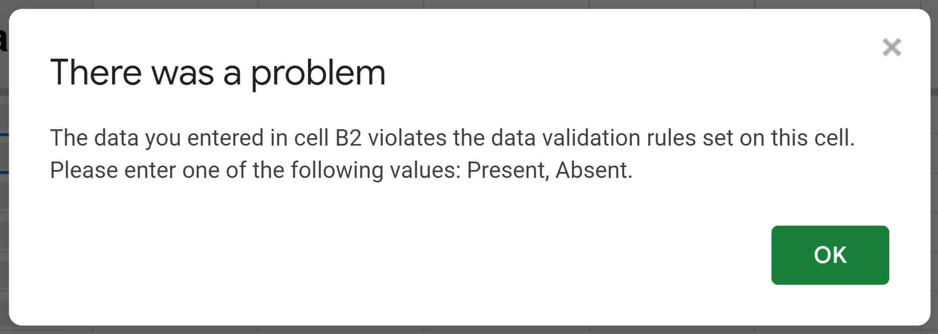
The second option is “Reject the input.” With this selected, when invalid data is entered, Google Sheets will reject the input, and a message will pop up that says “There was a problem”. You can see this demonstrated in the images below.
How to edit a drop-down / data validation
To edit the data validation for an existing drop-down, simply select the cell / range of cells that you want to edit the data validation of, and then open the data validation menu as described in the examples above, by clicking “Data” and then clicking “Data validation”. Then modify any settings that you want, and then click “Done”.
How to copy drop-down lists to other cells, and down the column
As mentioned earlier, if you specify a range of cells in the “Apply to range” field of the data validation menu, the drop-down lists will be applied to the entire range of cells. But if you have a drop-down list in one cell that you want to copy / apply to other cells, you can do this easily by copying and pasting a cell that contains a drop-down. You can also use “Autofill” to do this.
If you copy a cell that has a drop-down in it, you can paste it into another cell, and the drop-down will be applied to the cell where you pasted. As shown below, when you copy a cell, a dotted line will appear around the border of the cell.
To copy a drop-down in Google Sheets, select a cell that has a drop-down in it, press Ctrl + C on the keyboard to copy the cell, then select the cell / range of cells where you want to copy the drop-downs to, and then press Ctrl + V on the keyboard.
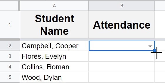
You can also use Autofill to copy drop-downs. As shown below, when you hover your cursor over the bottom right of the selected cell, the “Fill Handle” appears, which looks like a plus sign. When the fill handle appears, click, hold the click, and drag your cursor downwards until you reach the end of where you want your drop-downs, then release your click.
After either copying and pasting or using autofill to copy your drop-downs, the entire range that you pasted into / filled will have drop-down lists, as shown below.
Remove drop-down lists and data validation
So now that you know how to create drop-down lists, let’s go over how to remove them. There are four different ways to remove drop-downs / data validation in Google Sheets.
The first method, which is a new feature, is to simply press “Backspace” or “Delete” while the cell is empty and the dropdown menu / data validation will be removed.
You can also remove dropdowns / data validation by opening the data validation menu, and clicking the rule that you want to remove, and then click “Remove rule”.
Another method is this: After opening the data validation menu, hover your cursor over the rule that you want to remove, and on the right a garbage can icon will appear… click this and that rule will be removed.
You can also copy a cell that does not have a drop-down in it, and then paste it into the cell that contains the drop-down you want to remove.
To remove a drop-down in Google Sheets, select the cell or range of cells that contains the drop-down, then on the top toolbar click “Data”, and then click “Data validation”. Click the rule that you want to remove, then click the button that says “Remove rule”.
As you can see in the image above, a drop-down list is present in cell B2.

But after following the instructions above, the drop-down list is removed from cell B2, as shown below.
Quickly remove drop-down menus
A method that you can use to quickly remove drop-down menus from your spreadsheet, is to simply delete them by using the “Delete” or “Backspace” keys on the keyboard. To do this the cells must be empty in the first place.
If you want to delete a drop-down menu from a cell that has text in it, you’ll need to press “Backspace” once to delete the values from the cell, and then when you press “Backspace” again the drop-down menu will be deleted from the cell, and the cell will no longer be linked to the data validation rule.
If you do this for the entire range of cells that the data validation rule is applied to, the entire data validation rule will be removed.
But again this only works if the cells are empty, so this method is not good if you want to keep the values in the cells and remove only the data validation. Also, note that this does not work for all types of data validation.
Clearing all formatting to remove data validation
If you want you can use the “Clear formatting” feature to remove drop-down menus and data validation, but note that this will clear all of the formatting from a cell, including fill color, text formatting, etc.
Create a drop-down from another sheet
If you want, you can create a drop-down list where the drop-down and the criteria list are on different sheets.
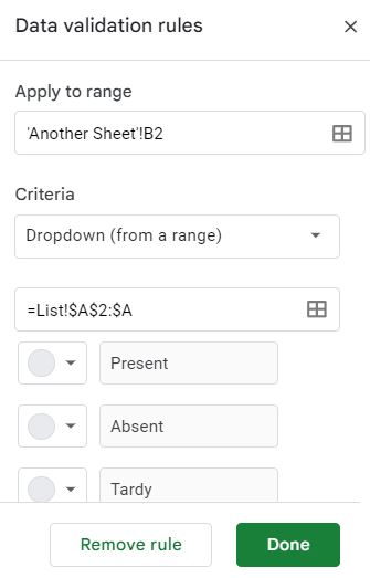
In the image below you can see that the criteria list / the list of items to use for the drop-down, is on its own tab, in column A. For this example, this tab with the list will be named “List”.
Follow the same normal process of creating a drop-down like in the previous examples. Select the cell / range of cells where you want to create your drop-down list(s), then click “Data”, then click “Data validation”, add a new rule, then choose “Dropdown (from a range)”. But in this case, enter (or select) a criteria range that refers to column A on the tab named “List”. As you can see in the image below, the cell range is: List!A2:A5
Click “Done”.
The cell address / range above refers to cells A2 through A5, from the tab named “List”. The exclamation point that appears after the word “List” is used to specify that we are referring to a tab name. In other words, to refer to a range on another sheet, type the name of the tab, then type an exclamation point, and then type the address for the range of cells containing the list for your drop-down.
Note that in the image below, the “Apply to range” field, and the criteria range are referring to different tabs. The drop-down will be on one sheet, and the list of items will be on a different sheet named “List”
As you can see in the image below, after applying the data validation settings shown above, a drop-down list was created on one tab, where the drop-down refers to a list on a different tab.
This content was originally created by Corey Bustos / SpreadsheetClass.com
Color cells based on drop-down selection (Conditional Formatting)
If you want, you can apply automatic color coding to your drop-down lists, where the color of the cell will be based on the drop-down selection. This is done by using “Conditional Formatting”.
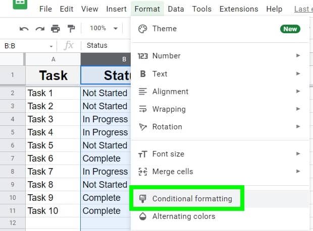
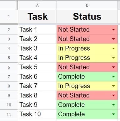
In the image below, we have a sheet with drop-down lists in it. Column A shows a list of tasks, and column B has drop-downs that have already been filled in, which show the status of each task (Not Started, In Progress, or Complete).
After your drop-downs are created, select the range of cells that contain your drop-downs, then click “Format” on the top toolbar, and then click “Conditional formatting”.
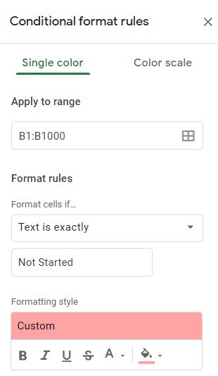
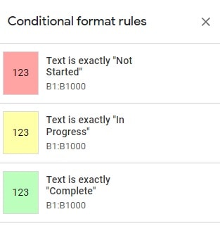
Create a conditional format rule, as shown below. For this example, we are formatting the cells with a light red background if the text in the cell says “Not Started”.
Create additional rules for each item in your list, as shown below. In this example we are making the cell background yellow if the text in the cell says “In Progress”, and we are making the cell background green if the text in the cell says “Complete”.
Below you can see what the conditional formatting does, after applying the rules mentioned above. Google Sheets automatically colors the cells in column B, based on the selection of the drop-down lists.
Pop Quiz: Test your knowledge
Answer the questions below about drop-down lists in Google Sheets, to refine your knowledge! Scroll to the very bottom to find the answers to the quiz.
Question #1
Which of the following settings will allow you to list the drop-down items in spreadsheet cells?
- Dropdown
- Dropdown (from a range)
Question #2
Which of these options will allow you to specify the list of items for the drop-down directly in the data validation menu?
- Dropdown
- Dropdown (from a range)
Question #3
True or False: You can apply data validation to multiple cells at once, and you can copy drop-downs / data validation from one cell to another
- True
- False
Question #4
True or false: The “Apply to range” field refers to the range that the data validation is being applied to
- True
- False
Question #5
True or False: The “Criteria” range refers to the cells where the list of items are entered (When using “List from a range”)
- True
- False
Answers to the questions above:
Question 1: 2
Question 2: 1
Question 3: 1
Question 4: 1
Question 5: 1