

In Google Sheets, many know how to highlight a cell based on its value, by using conditional formatting. But did you know that you can use conditional formatting to highlight an entire row based on the value of a single cell? That’s what I’m going to show you how to do in this lesson.
To highlight a row based on a cell value, follow these steps:
- On the top toolbar, click “Format”, then click “Conditional formatting”
- Click “Add another rule”
- Under the “Format rules” section, under the drop-down that says “Format cells if”, select “Custom formula is”
- In the blank field below, enter the following formula =$A1=”Yes” (This will highlight the entire row if the value in cell A1 is “Yes”)
- Press “Enter” on the keyboard
- (Optional) Choose the color / format that you want the highlighted rows to be (Fill color)
Click here to get your free Google Sheets cheat sheet
Highlight row based on cell value
To highlight a row based on a cell value, we need to use the “Custom formula is” option in the conditional formatting menu. “Custom formula is” allows you to specify which cells to format based on a specified criteria / formula.
On the top toolbar, click “Format”
Then click “Conditional formatting” and a menu will pop up on the right
Click “Add another rule”.
In the “Apply to range” field, type A1:Z1000 and press “Enter” on the keyboard. If we had selected this range of cells before opening the conditional formatting menu, Google Sheets would have automatically filled in the cell range for us.
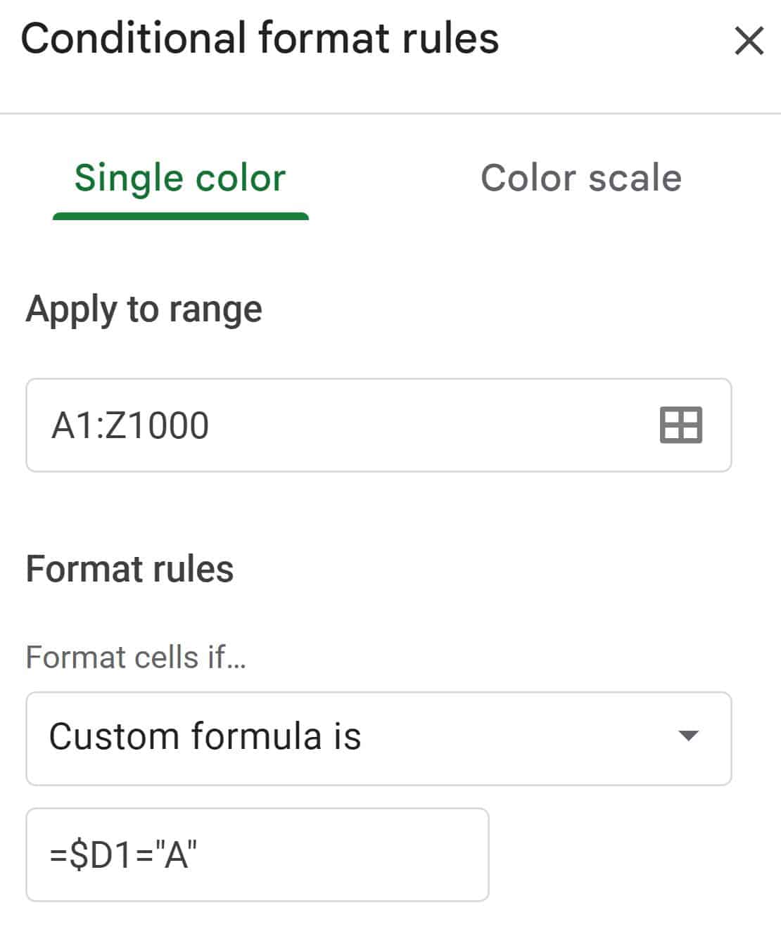
Click the “Format cells if” dropdown, and choose “Custom formula is”
Then type the formula =$D1=”A” and press “Enter” on the keyboard. This formula tells Google Sheets to format / highlight the rows where column D is equal to “A”. In other words, it highlights the rows where the letter “A” is found in column D.
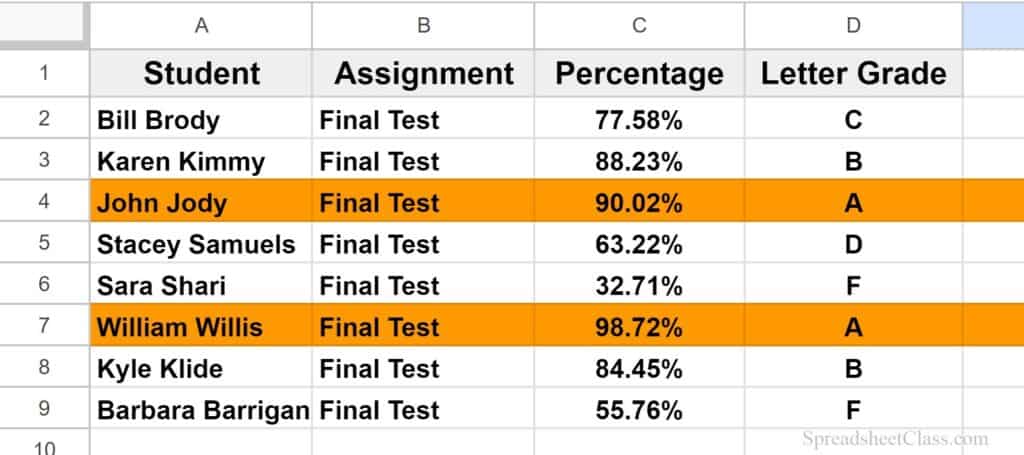
As you can see in the example image further below, this highlights the rows for the students who received a letter grade of “A” on their assignment.
Apply to range: A1:Z1000
Custom formula is: =$D1=”A”
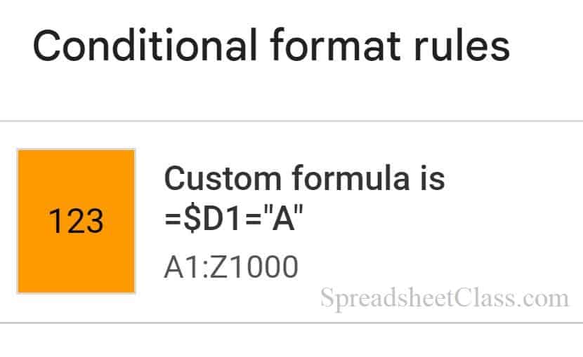
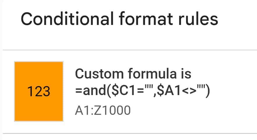
The image above shows what the conditional formatting rule will look like, when the rule is open / being edited. The image below shows that the conditional formatting rule looks like in the main conditional formatting menu where all of the rules are displayed. Note that the bottom part of the rule displays the “Apply to range” field, and the top part shows the custom formula.
In this example I have chosen an orange “Fill color” / background color for this conditional formatting rule.
After following the steps above, when the letter “A” is found within column D, that row will be highlighted, as shown in the image below.
Highlight row based on date
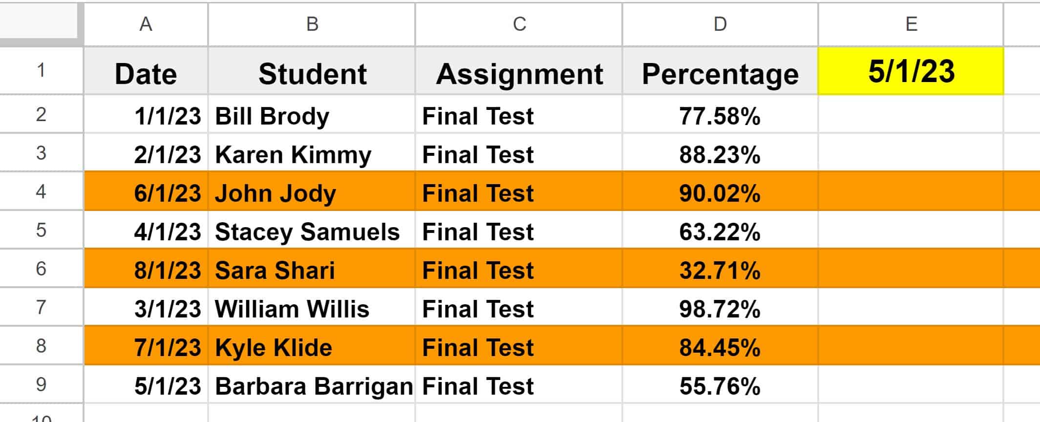
In this example we will highlight an entire row based on a date, where the rows will be highlighted if the date is greater than (later than) a specified date. We will use the same method from the previous example, but we will simply make a small change to our “Custom formula is” formula.
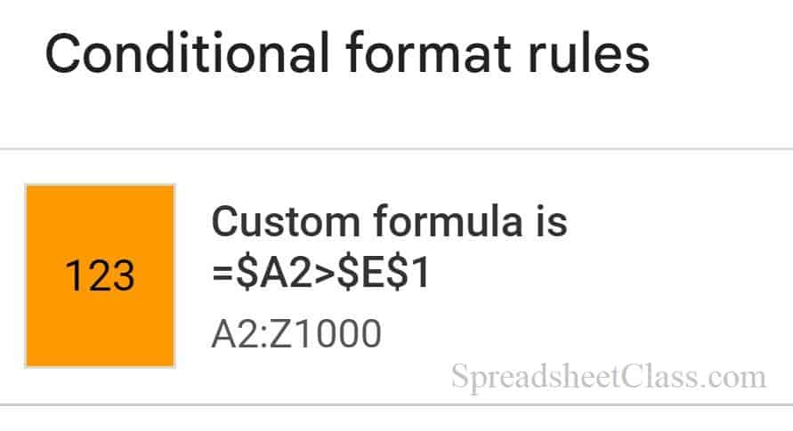
In this case, we want to highlight the row(s), if the dates in column A are greater than the date entered in cell E1.
Apply to range: A2:Z1000
Custom formula is: =$A2>$e$1
Follow the same steps from the previous example:
Open the data validation menu, add a new rule, select “Custom formula is”, then enter the following formula: =$A2>$e$1
In the “Apply to range” field, if the range A2:Z1000 is not already entered, type the range and then press “Enter”
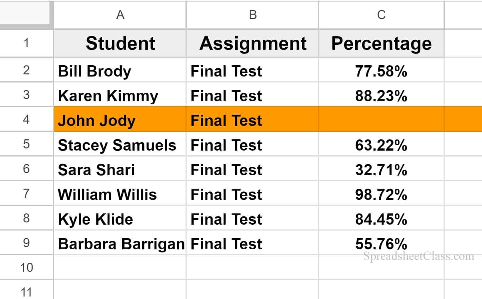
After following the steps above, in column A if the date in the cell is greater than / later than the date entered in cell E1, that row will be highlighted, as shown in the image below. For example, in row 4, the date in cell A4 is later than the date entered in cell E1, and so row 4 is highlighted.
Highlight row if cell is empty
Sometimes you might want to highlight an entire row if a cell in the row is empty. Again we will make a small change to the “Custom formula is” formula, to do this.
In this case we want to highlight the entire row wherever there is a blank cell in column C.
Apply to range: A1:Z1000
Custom formula is: =$C1=””
Follow the same steps from the previous example:
Open the data validation menu, add a new rule, select “Custom formula is”, then enter the following formula: =$C1=””
In the “Apply to range” field, if the range A1:Z1000 is not already entered, type the range and then press “Enter”
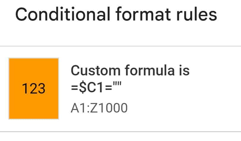
After following the steps above, wherever there is a blank cell in column C, that row will be highlighted, as shown in the image below.
Highlight row if cell is NOT empty
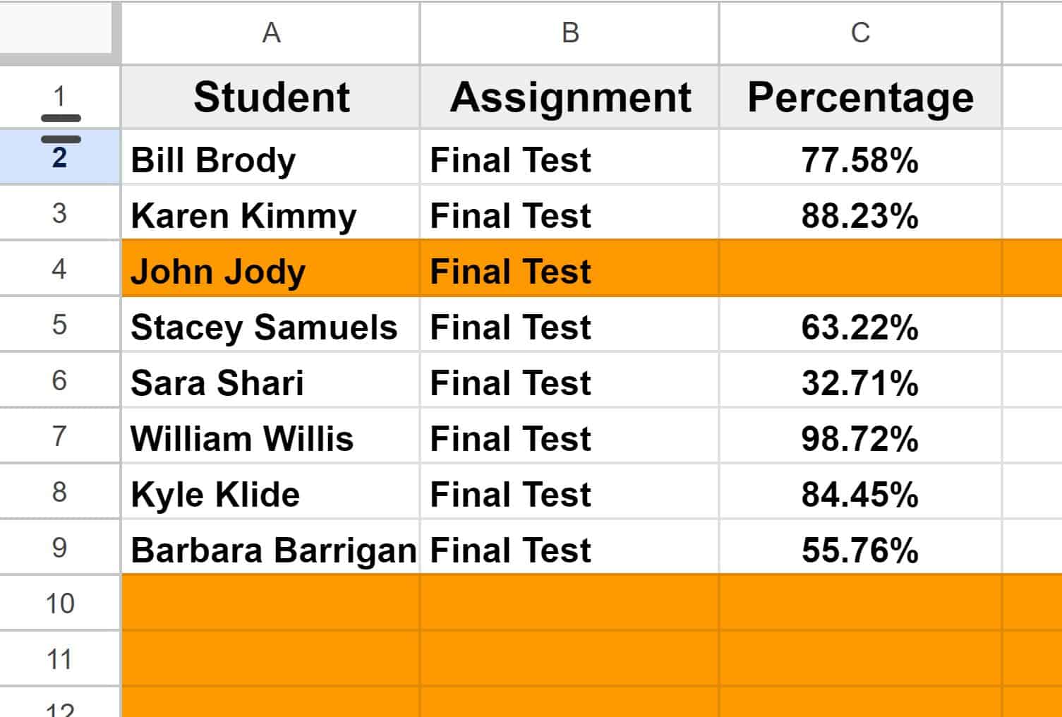
Now let’s do the opposite of the last example. Sometimes you might want to highlight an entire row if a cell in the row is NOT empty. We will make a slight change to the “Custom formula is” formula, to do this.
In this case we want to highlight the entire row wherever there is NOT a blank cell in column C, i.e. if the cell has anything inside it, it will be highlighted.
Apply to range: A2:Z1000
Custom formula is: =$C2<>””
Follow the same steps from the previous example:
Open the data validation menu, add a new rule, select “Custom formula is”, then enter the following formula: =$C2<>””
In the “Apply to range” field, if the range A2:Z1000 is not already entered, type the range and then press “Enter”
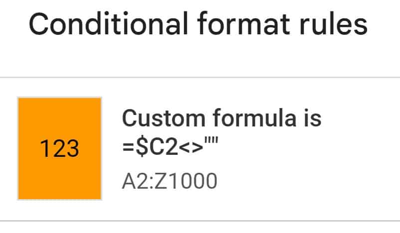
After following the steps above, in any row that has a non-blank cell in columnC, that row will be highlighted, as shown in the image below.
Highlight row if cell is empty (Ignore blank rows)
In this last example, we will go over how to highlight a row if a cell is empty, but we will ignore rows that are completely blank. In this example we will assume that if a cell in column A is blank, the entire row is blank.
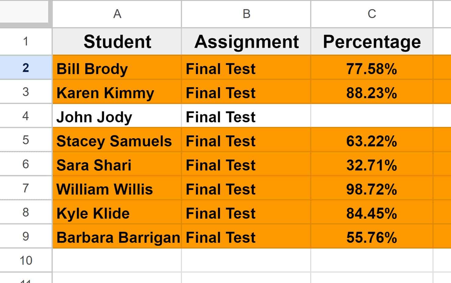
We are going to tell Google Sheets to highlight rows where column A is not blank, and where column C is blank.
Apply to range: A1:Z1000
Custom formula is: =and($C1=””,$A1<>””)
Follow the same steps from the previous example:
Open the data validation menu, add a new rule, select “Custom formula is”, then enter the following formula: =and($C1=””,$A1<>””)
In the “Apply to range” field, if the range A1:Z1000 is not already entered, type the range and then press “Enter”
After following the steps above, in the rows where column C is blank and column A is not blank, those rows are highlighted, as shown in the image below. This will prevent completely blank rows from being highlighted when you are only interested in rows that actually have data in them.
Now you know how to highlight entire rows based on cell values in Google Sheets!
Click here to get your free Google Sheets cheat sheet
This content was originally created by Corey Bustos / SpreadsheetClass.com