7 ways to highlight duplicates in Google Sheets

When you're using Google sheets, sometimes you'll have duplicates in your data and you'll want a way to highlight them so that you can easily see where they are.

In this lesson I'm going to show you several ways to highlight duplicates in Google sheets. You'll learn how to highlight duplicates in a single column, across an entire sheet, and more.

Now the duplicates on your spreadsheet (Column A in this example) will be highlighted!

Check out this lesson if you want to learn how to remove duplicates in Google Sheets instead of highlighting them.

You can also learn how to remove duplicates with a formula in this lesson.

Click here to get your Google Sheets cheat sheet

Method 1: Highlight duplicates with conditional formatting (custom formula is)

The most common way to highlight duplicates in Google Sheets, is by using the “Custom formula is” option in the conditional formatting rules.

“Custom formula is” allows us to use a formula to specify which cells to format based on a specified criteria, such as telling Google Sheets to format the values that are counted more than once (i.e. duplicates).

Highlight duplicates in a single column

In this example, we are going to highlight duplicate names within a single column, again by using conditional formatting.

Note that you can specify the range that you want to apply the conditional formatting to in two different ways.

The first is by selecting the range that you want to format before opening the conditional formatting menu, and Google Sheets will automatically fill in the cell range…

Or you can simply open the "Conditional formatting” menu and type the range that you want to apply the formatting to, under the ”Apply to range” field.

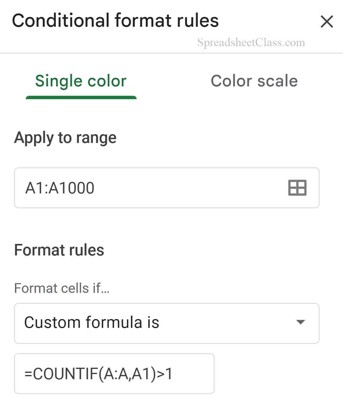
In this example the names are listed in column A, and so we will select column A before opening the Conditional formatting menu, or alternatively you can simply open the menu and then type the range A1:A1000 in the “Apply to range” field

On the top toolbar, click "Format", and then click "Conditional formatting"… and then click "Add another rule".

Notice that in the "Apply to range" field, Google Sheets has filled in the cell range for us (A1:A1000) because we selected this range before opening the menu, but this range can also be typed manually if you want.

Then click the "Format cells if" dropdown, and choose "Custom formula is"

Then type the formula =COUNTIF(A:A,A1)>1 and press "Enter" on the keyboard. This formula tells Google Sheets to format the cells in column A that appear / are counted more than once.

Apply to range: A1:A1000

Custom formula is: =COUNTIF(A:A,A1)>1

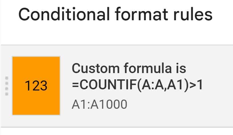
In this example I have chosen an Orange fill color (background color) for the conditional formatting rule, and as you can see in the image below, after following the steps above, the duplicate names in column A are now highlighted in orange.

Note that the conditional formatting rule above (in the main conditional formatting menu where all of the rules are displayed), the custom formula is shown on top, and the range that the formatting is applied to, is shown on bottom.

Highlight duplicates found within multiple columns

Now let's go over an example where there are multiple columns of data, and duplicates that appear across multiple columns. For example let's say you have two columns of names, and you want to highlight any and all duplicate names that appear in those two columns.

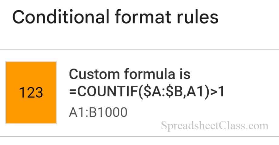
Doing this is very simple. We need to make a slight change to the range the formatting is being applied to, and a slight change to the "Custom formula is" formula, so that we are referring to two columns instead of one, like this

Apply to range: A1:B1000

Custom formula is: =COUNTIF($A:$B,A1)>1

Notice that I also included dollar signs before the letters in the range that we are referring to, these are needed to make sure the formula works correctly.

Follow the same steps from the previous example:

Open the data validation menu, add a new rule, select "Custom formula is", then enter the following formula: =COUNTIF($A:$B,A1)>1

In the "Apply to range" field, if the range A1:B1000 is not already entered, type the range and then press "Enter"

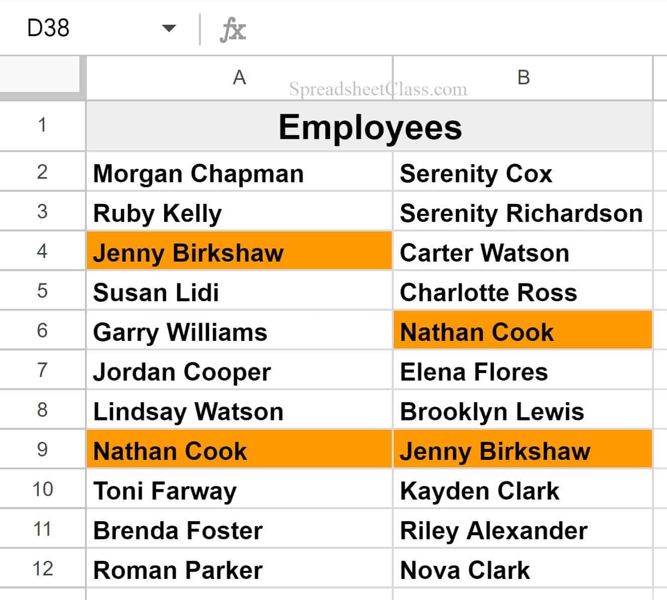
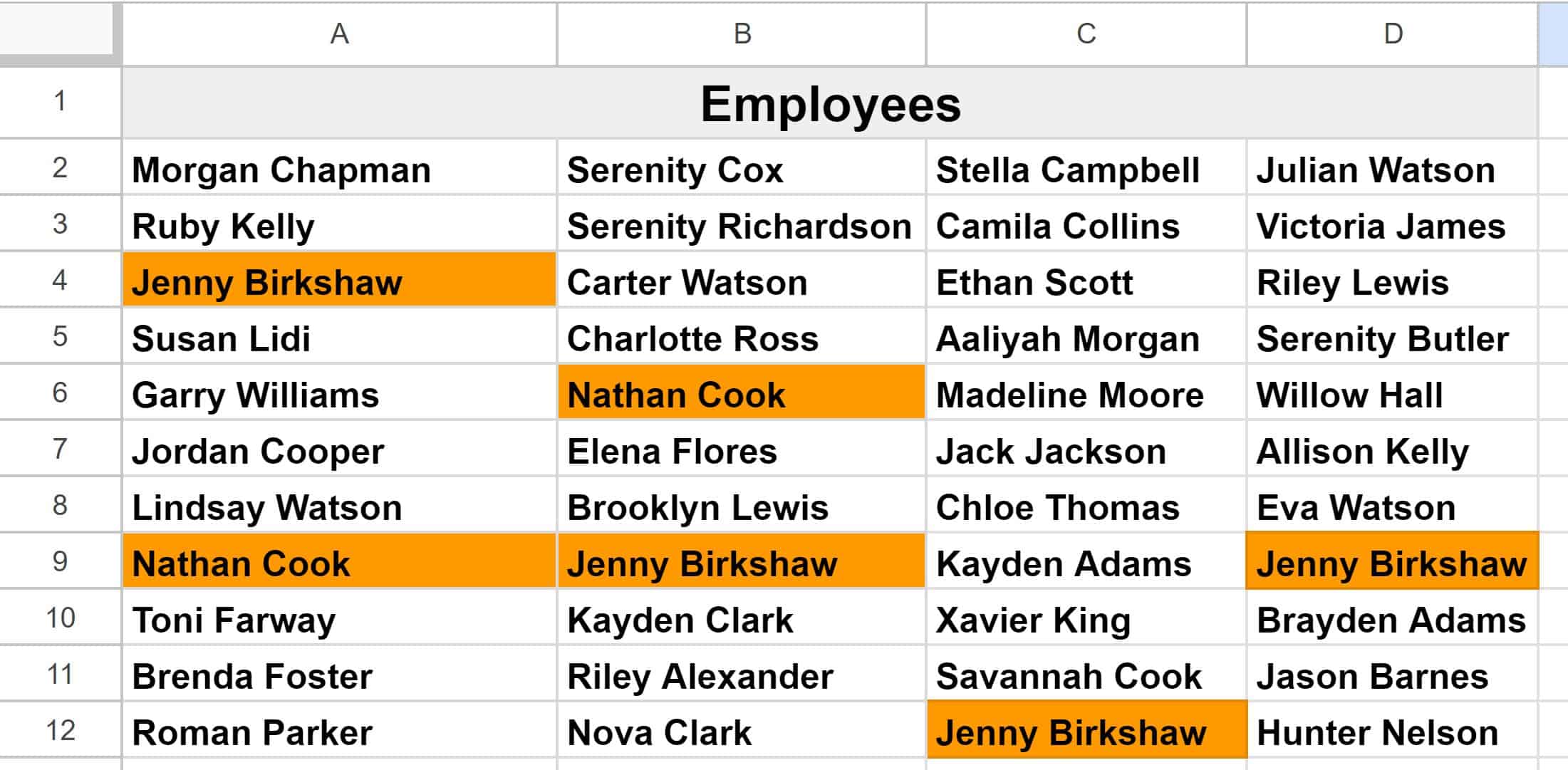
After following the steps above, the duplicate names listed in two columns will be highlighted, as shown in the image below. For example, "Nathan Cook" appears once in column A, and once in column B, and so both are highlighted because they are duplicates while using the formula to search through both columns.

Highlight duplicates found within an entire sheet

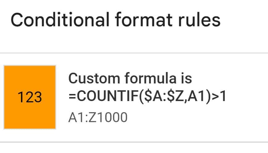
You can also highlight duplicates across an entire sheet, by using the same method from the previous example, but instead of referring to two columns, in this case we will refer to columns A through Z.

Apply to range: A1:Z1000

Custom formula is: =COUNTIF($A:$Z,A1)>1

Follow the same steps from the previous example:

Open the data validation menu, add a new rule, select "Custom formula is", then enter the following formula: =COUNTIF($A:$Z,A1)>1

In the "Apply to range" field, if the range A1:Z1000 is not already entered, type the range and then press "Enter"

After following the steps above, the duplicate names listed in your entire spreadsheet will be highlighted, as shown in the image below.

Highlight entire row when duplicate is found

Another way that you can highlight duplicates is by highlighting an entire row when a duplicate is found within a single column. This simply requires a different formula under the “Custom formula is” section in the conditional formatting menu. In this case we are going to refer to multiple columns in the "Apply to range" field, and we will refer to a single column in the custom formula, but this time we will include a dollar sign before "A1" (The criteria to search for in the COUNTIF function.) like this: =COUNTIF($A:$A,$A1)>1

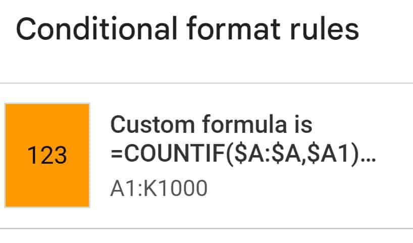
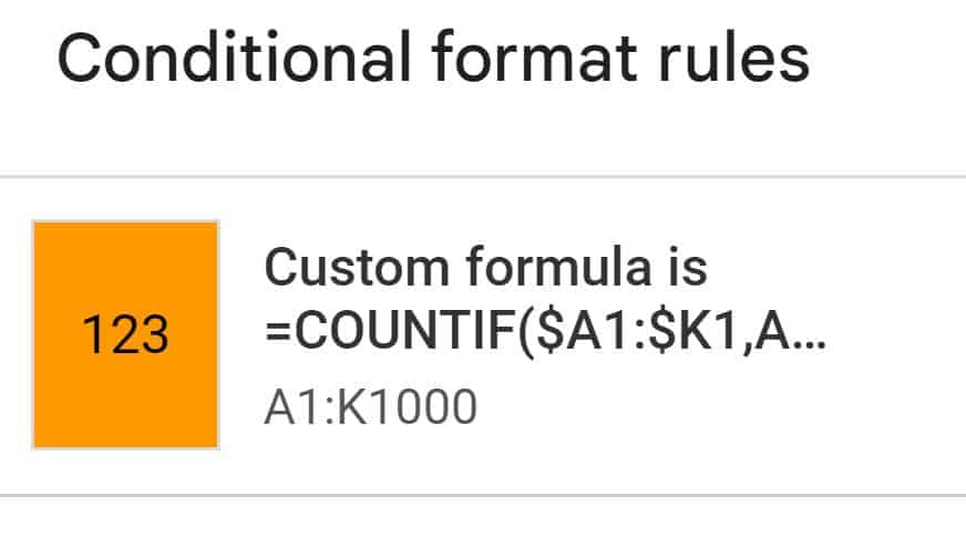
Apply to range: A1:K1000

Custom formula is: =COUNTIF($A:$A,$A1)>1

Follow the same steps from the previous example:

Open the data validation menu, add a new rule, select "Custom formula is", then enter the following formula: =COUNTIF($A:$A,$A1)>1

In the "Apply to range" field, if the range A1:K1000 is not already entered, type the range and then press "Enter"

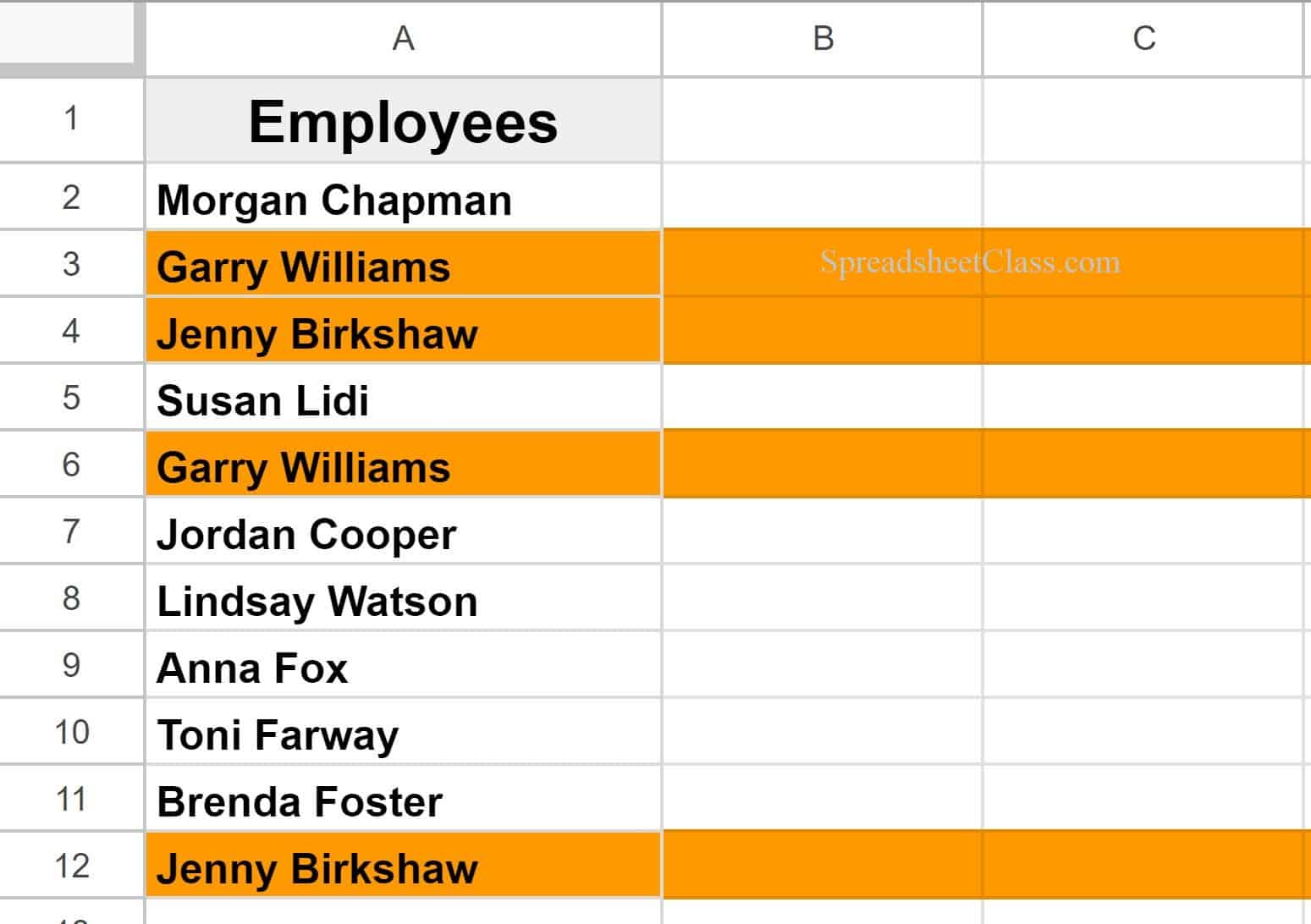
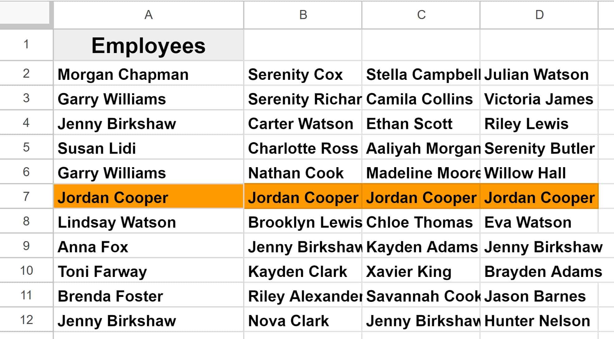
After following the steps above, the entire row that the duplicate names are found in, will be highlighted, as shown in the image below.

Highlight duplicate rows

If you want, you can have Google Sheets highlight an entire row if every value in the row is a duplicate. Let's say that you want to highlight the rows where each column has the same name, in the same row. To do this we will change the custom formula in the conditional formatting menu. In this case we are telling Google Sheets to highlight the row if the name is counted 4 times, like this:

(Highlights the row, only in the columns that the duplicates are found in) =COUNTIF($A1:$K1,A1)=4

(Highlights the entire row when duplicate criteria is met) =COUNTIF($A1:$K1,$A1)=4

Note that in the two formulas above, one has an extra dollar sign before the "A1" reference. This will highlight the entire row (as opposed to only highlighting where the duplicates are.)

Apply to range: A1:K1000

Custom formula is: =COUNTIF($A1:$K1,A1)=4

Follow the same steps from the previous example:

Open the data validation menu, add a new rule, select "Custom formula is", then enter the following formula: =COUNTIF($A1:$K1,A1)=4

In the "Apply to range" field, if the range A1:K1000 is not already entered, type the range and then press "Enter"

After following the steps above, the row / rows that the duplicate names are found in, will be highlighted, as shown in the image below.

Method 2: Using COUNTIF with cells in a column to detect duplicates

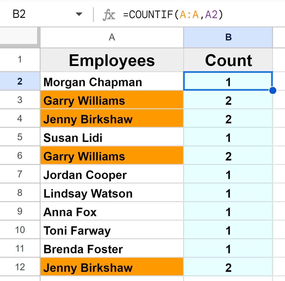
If you want, as an alternative method you can use the COUNTIF function to count how many times a certain value is found within a column, as a simple indicator of which values have duplicates (i.e. If a value is duplicated then the COUNTIF function will display a number higher than 1.) With this method you can see how many times a certain value is duplicated, and not just the fact that it is / is not a duplicate.

This method also uses the "custom formula is" option in the conditional formatting menu if you want to highlight the duplicate items directly, but if you wanted you could simply highlight the numbers in the column that contains the COUNTIF function, so that any number greater than 1 is highlighted. But again if you want the duplicated text itself to be highlighted, you must still use "custom formula is" as demonstrated below. Although "custom formula is" is still required, this method is easier and more intuitive when it comes to the custom formula entered into the conditional formatting rule.

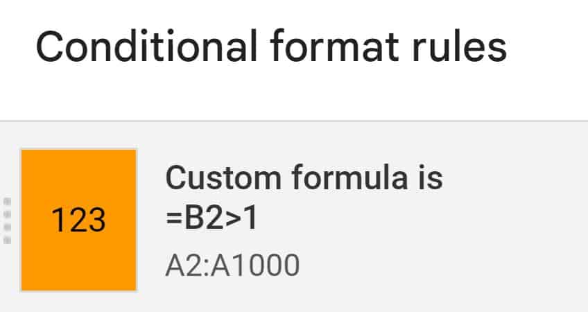
Notice the formula in this example for the "Custom formula is" option, is =B2>1

This custom formula / rule simply tells Google Sheets to highlight cells (in column A) where the cells in column B are greater than 1. So the formula in the spreadsheet cell counts how many times the value appears in the list… and the custom formula in the conditional formatting rule tells Google Sheets to highlight cells in column A if the cells in column B are greater than 1 (i.e. duplicates).

Apply to range: A1:A1000

Custom formula is: =B2>1

After following the steps above, the cells that the duplicate names are found in, will be highlighted, as shown in the image below.

This content was originally created by Corey Bustos / SpreadsheetClass.com

Highlight duplicates from another sheet

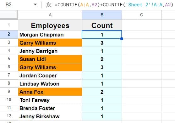
Conditional formatting formulas cannot refer to another tab, and so if you have duplicates from two sheets that you want to highlight, you can use the method in the previous example (Using the COUNTIF function in the column beside your data to count / check for duplicates), but this time we will using the following formula to count how many times each name appears on the first tab, and then we will add this number to how many times the name is found in another tab: =COUNTIF(A:A,A2) + COUNTIF('Sheet 2'!A:A,A2)

So we are adding one COUNTIF function to another one, where the first part of the formula counts how many times the name appears in column A, and the second part of the formula counts how many times the name appears on Sheet 2 (and the numbers are added together).

The same conditional formatting rule / formula from the previous example is used: =B2>1

Apply to range: A1:A1000

Custom formula is: =B2>1

See how in the image below, the names "Susan Lidi" and "Anna Fox" are highlighted, even though their name only appears once on the first tab… this is because their name appears on Sheet 2 as well.

Now you know all the different ways to highlight duplicates in Google Sheets!

Click here to get your Google Sheets cheat sheet