How to use the SORT & SORTBY functions in Excel

The SORT function is an incredibly useful formula that you can use to sort your data in Microsoft Excel. With the SORT function you can sort your data by a specified column (or multiple columns), in ascending or descending order, and you can also sort data vertically or horizontally.

The sort function can be used to sort data alphabetically (A-Z), or numerically.

In this lesson I am going to show you how to do all of these things with the Excel SORT function. I will also teach you how to sort by multiple columns with the SORTBY function.

Using the SORT function in Excel is similar to using it in Google Sheets, but there are some differences between the two. Click here to read the Google Sheets version of this article

SORT formulas for Excel:

Here are the types of SORT and SORTBY formulas that I am going to teach you in this lesson. Further below are examples of how to use each of these formulas.

Click here to get your Google Sheets cheat sheet

The Microsoft Excel SORT function:

These diagrams will show you how to set up your SORT function, and will show you what each component of the formula does, so that you can understand how to use the SORT function for custom tasks.

The SORT function works by specifying a range to be sorted, then the column number to sort by, and then the order to sort by (Ascending / Descending), and then you specify whether to sort by row (vertical sort) or by column (horizontal sort).

=SORT(A3:C100,1,1,FALSE)

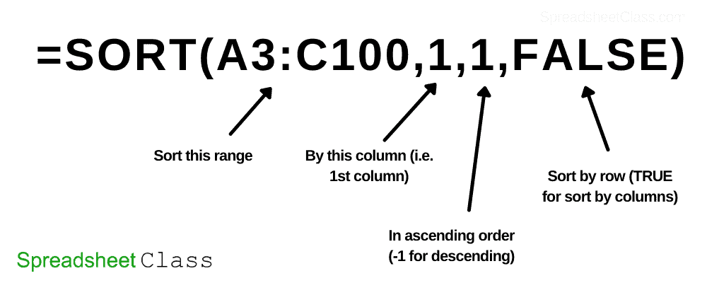
Setting the column number

When specifying the column to sort by in your SORT function, type a number that represents the position of the column that you want to sort by, in reference to the range that you specified.

For example, if you are sporting the range A2:C100, and you want to sort by column B, then this is column "2" in the range that you are sorting by. Much the same, column C would be "3".

However if you are sorting range B2:Z100, and you want to sort by column B, this would be designated as column "1", as it is the first column in the range that you specified.

The default setting for the SORT function is to sort by the first column.

Setting the sort order (Ascending vs. descending)

When specifying the order to sort by in your SORT function, choose one of the following options:

• 1 (Ascending)
• -1 (Descending)

So a positive number 1 means ascending, and a negative number 1 means descending. The default setting for the SORT function is to sort in ascending order.

Setting the option to sort by row or sort by column

When specifying whether to sort by row or sort by column in your SORT function, choose one of the following options:

• FALSE (Sort by row)
• TRUE (Sort by column)

The default setting for the sort function is to sort by row.

The Excel SORT function description:

Syntax:
=SORT(array,[sort_index],[sort_order],[by_col])

Formula summary: “Sorts a range or array”

Later I will go into detail about how to use the SORTBY function, but let's start off by using the SORT function.

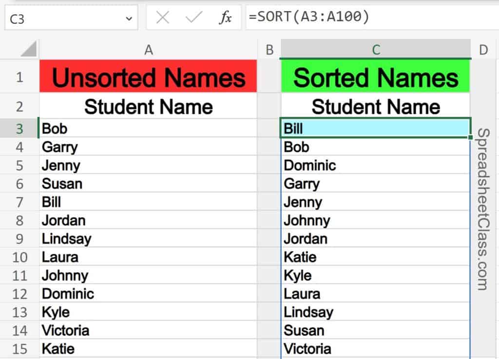
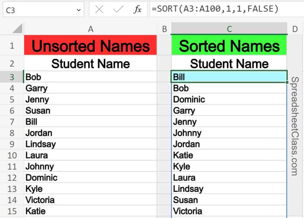
Sorting a single column in ascending order

First, I am going to show you how to sort a single column of data, in ascending order, with the SORT function.

When you want to sort by the first column in ascending order, you don't have to specify anything other than the range to sort, in the SORT function. You will see that both of the formulas below do the same thing, where one has the column and order to sort by etc. specified, and the other doesn't.

In other words if you don't specify a column number, sort order, or to sort by rows / columns, then Excel will sort by the first column, in ascending order, by row.

Notice that in this example the data is all text, and so the data will be sorted alphabetically.

The task: Sort the list of names in column A, from A to Z

The logic: Sort column A (A3:A100) in ascending order

The formula: The formula below, is entered in the blue cell (C3), for this example

=SORT(A3:A100)

Formula with same functionality: =SORT(A3:A100,1,1,FALSE)

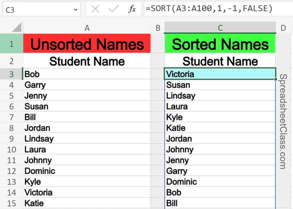
Sorting in descending order

In this example we will sort the same list of names in descending order (Z to A), by changing "1" to "-1" in the formula.

The task: Sort the list of names in column A from Z to A

The logic: Sort column A (A3:A100) in descending order

The formula: The formula below, is entered in the blue cell (C3), for this example

=SORT(A3:A100,1,-1,FALSE)

Sorting by multiple columns

Now I'll show you how to use the SORTBY function to sort by multiple columns in Excel. To do this you will specify the range to sort, then the first column that you want to sort by (designated as a range), then the order, and then you will do the same thing for the next column that you want to sort by.

So with the SORTBY function, instead of typing the number of the column to sort by (like in the SORT function), you will specify the column(s) to sort by by typing the range for the column(s) to sort by.

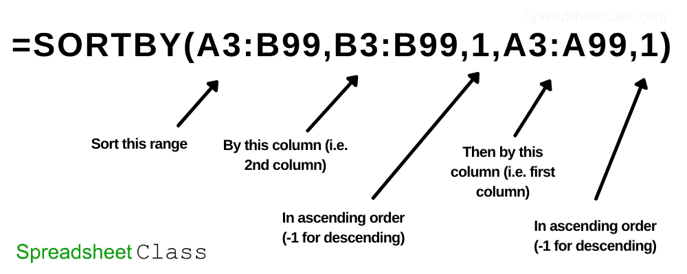
Excel SORTBY function diagram (Sort by multiple columns):

This diagram shows a formula that sorts by 2 columns, where the first specified column sorts in ascending order, and the second specified column sorts in ascending order.

=SORTBY(A3:B99,B3:B99,1,A3:A99,1)

The Excel SORTBY function description:

Syntax:
=SORTBY(array, by_array1, [sort_order1], [by_array2, sort_order2],…)

Formula summary: “Sorts a range or array based on the values in a corresponding range or array”

So the first column that is specified will be the priority… and then any sorting that can be done without interrupting the grouping created by the first column designation, will be done.

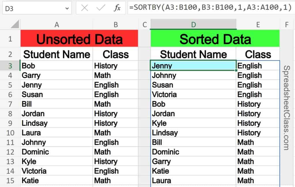
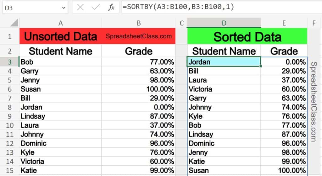
In this example we will sort a list of students and their classes by class first, and then by name.

The task: Sort by class, then by student name

The logic: Sort the range A3:B100, by column 2 in ascending order and then by column 1 in ascending order

The formula: The formula below, is entered in the blue cell (D3), for this example

=SORTBY(A3:B100,B3:B100,1,A3:A100,1)

Sorting by numerical values

So far we have used the SORT function to sort text alphabetically, but in this example you'll see that the SORT function can also sort numerical data in Excel.

(If your data has both numbers and text, numbers will sort first, and then letters after)

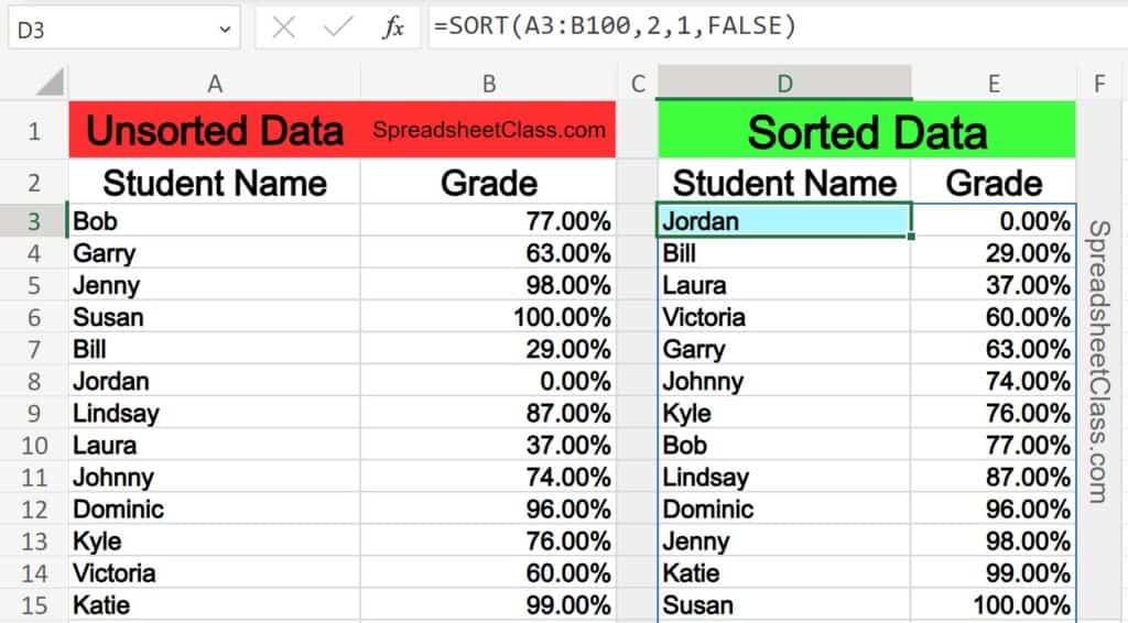
This first part of the example shows a list of students and their grade percentage, sorted with the lowest grades showing at the top of the list.

The task: Sort the student data by grade percentage

The logic: Sort the range A3:B100, by column 2 in ascending order

The formula: The formula below, is entered in the blue cell (D3), for this example

=SORT(A3:B100,2,1,FALSE)

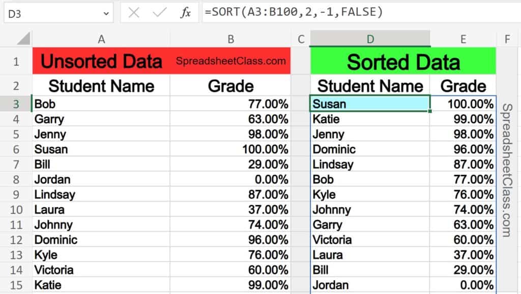
Here is the same example, sorted in descending order (Best grades on top).

=SORT(A3:B100,2,-1,FALSE)

Content originally created by Corey Bustos / SpreadsheetClass.com

Sorting by a range instead of a column number

If you would like, instead of entering a column number to specify the column that you want to sort by, you can use the SORTBY function to enter the range of the column that you want to sort by. For example, let's achieve the same task as the formula in the example above, but we will specify a range rather than a column number, by using the SORTBY function. Note that the two formulas below will do the same thing.

=SORT(A3:B100,2,1,FALSE)

=SORTBY(A3:B100,B3:B100,1)

The first formula refers to the second column which is column B, and the second formula refers to the range B3:B, which is again column B. Either way is an acceptable way to sort with a formula.

Note that the image below shows the same sorted results as in the example above, by using the SORTBY function instead of the SORT function.

Sorting by date

You can also sort data by date, by using the SORT function in Excel.

Dates in a spreadsheet are really just numbers, and so earlier dates are simply just smaller numbers than later dates, making it easy to use the SORT function to sort by date.

The task: Sort the list of dates from earliest to most recent

The logic: Sort the range A2:A100, by column 1 in ascending order

The formula: The formula below, is entered in the blue cell (C2), for this example

=SORT(A3:A100)

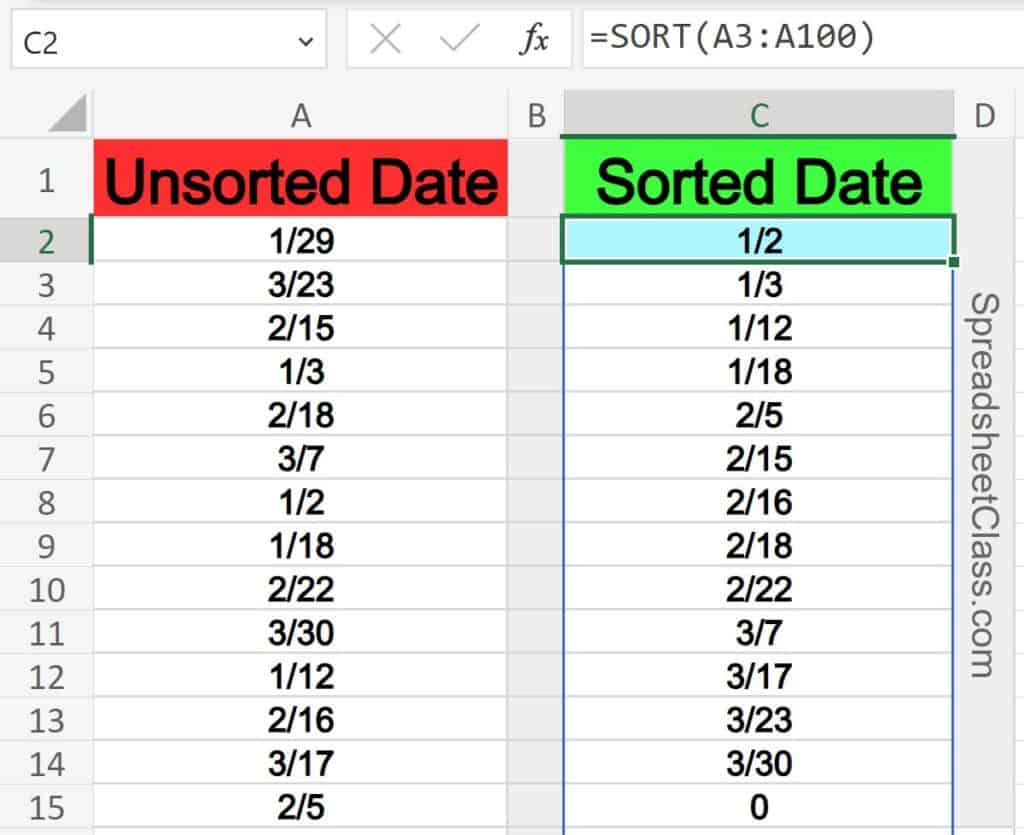
Note that in the example image above, the column number, and order to sort by etc. was not specified, because the default for this function is to sort by the first column, in ascending order, by row. This is what we wanted in this case, so no additional criteria was needed for the SORT function. But the formula below (which does specify the column / order to sort by), will do the same thing as the formula above.

=SORT(A3:A100,1,1,FALSE)

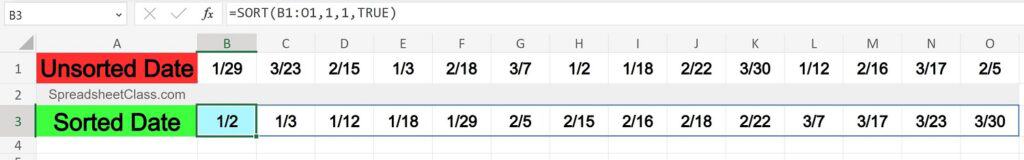
Sorting horizontally

You may find cases where you need to sort your data horizontally, and this can be done by using the SORT function, and choosing the sort by columns instead of by rows.

So far we have been choosing to sort by rows by specifying (FALSE) in the formula criteria that determines whether to sort by rows or columns. But now we will change this setting to (TRUE), to sort by columns, which will sort horizontally.

The example formula below horizontally sorts the horizontal list of dates.

The task: Sort the list of dates horizontally, from earliest to most recent

The logic: Sort the range B1:O1, by the first row in ascending order

The formula: The formula below, is entered in the blue cell (B3), for this example

=SORT(B1:O1,1,1,TRUE)

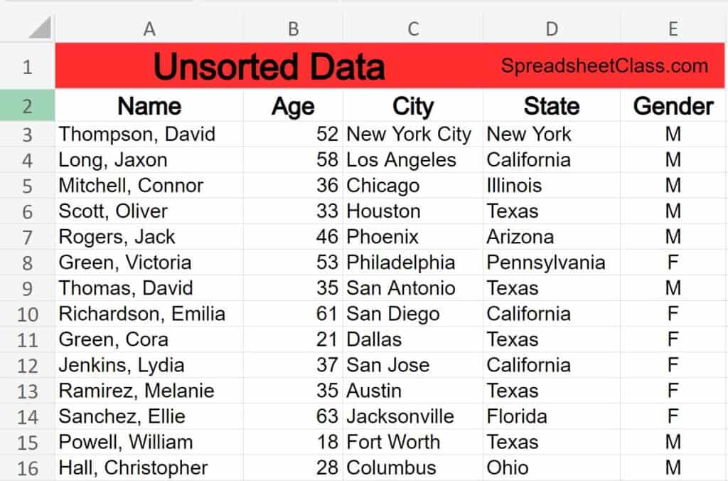
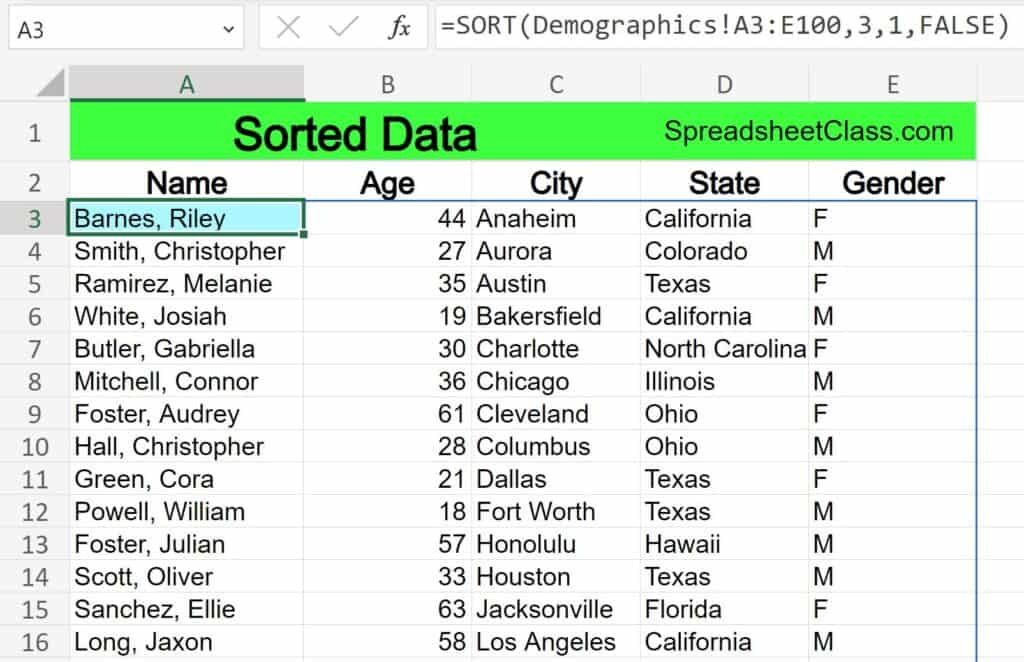
Sorting data from another tab

You may often find the need to sort data that is on another tab, where your formula output is on a tab that is separate from the tab that contains your source data.

This can be done by specifying the tab name in the data range for your SORT formula. To do this simply add the name of the tab that you want to reference as well as an exclamation point, before typing the range. For example, here we will reference the tab named "Demographics" and so our reference looks like this:

Demographics!A3:E100

If your tab name has a space in it, make sure to include apostrophes before and after the tab name, like this:

'Sheet 1'!A3:Z100

Let's take a look at an example of putting this into action.

The task: Sort the data on the "Demographics" tab, by city, from A to Z

The logic: Sort the range A3:E100, on the tab labeled "Demographics", by the third column in ascending order

The formula: The formula below, is entered in the blue cell (A3), for this example

=SORT(Demographics!A3:E100,3,1,FALSE)

This is the tab named "Demographics", where the source data is located:

This is the tab that contains the SORT formula:

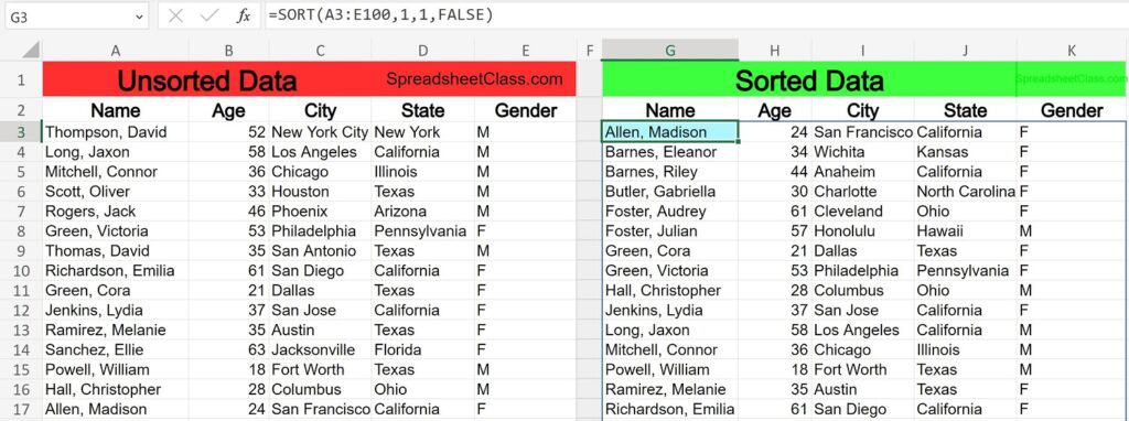
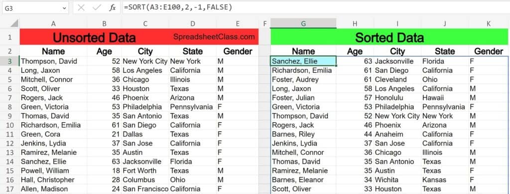
Here are some more examples of sorting this same data on a single tab, in a variety of ways, so that you can see how changing the formula parameters changes the formula output.

The formulas: The SORT and SORTBY formulas below, are entered in the blue cells (G3), for these examples

=SORT(A3:E100,1,1,FALSE)

Sorted by name in ascending order:

=SORT(A3:E100,2,-1,FALSE)

Sorted by age in descending order:

=SORTBY(A3:E100,D3:D100,1,C3:C100,1)

Sorted by state in ascending order, then by city in ascending order:

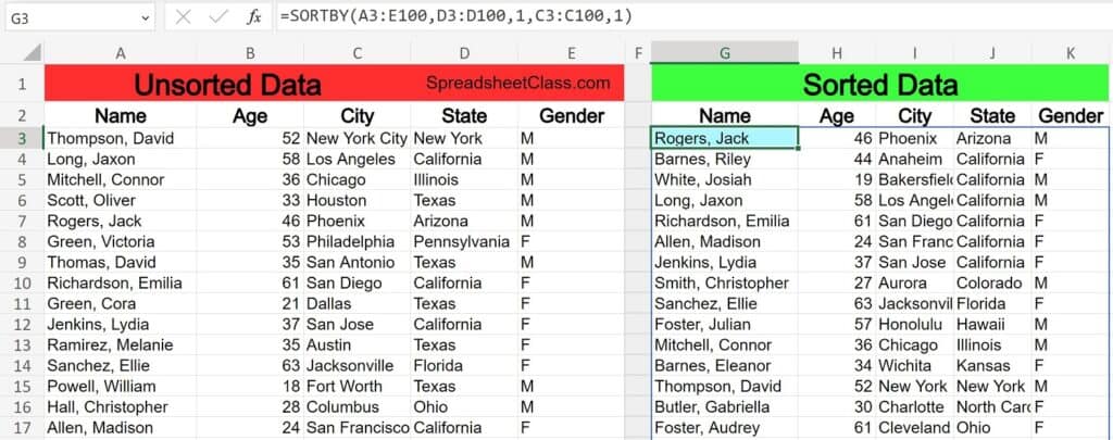
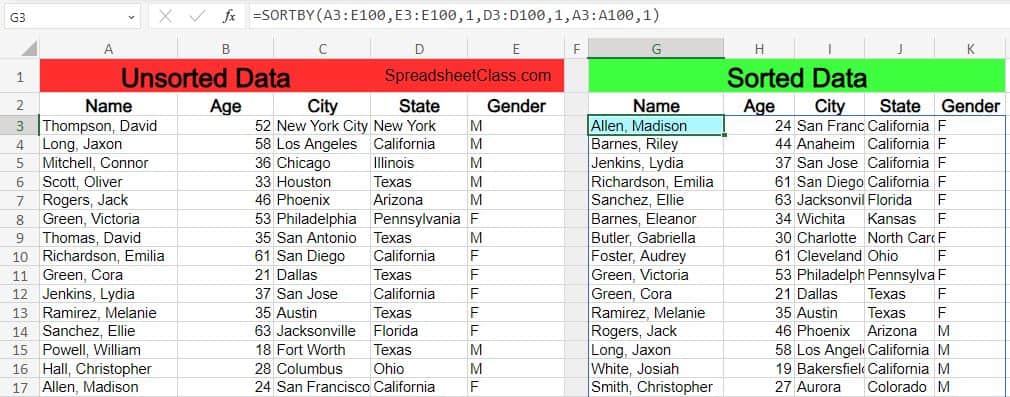
=SORTBY(A3:E100,E3:E100,1,D3:D100,1,A3:A100,1)

Sorted by gender in ascending order, then by state in ascending order, then by name in ascending order:

Using the SORT function with the FILTER function

In Excel, you can combine multiple functions into a single formula.

In the video below, you will learn how to use the SORT function with the FILTER function, as individual functions, and combined into one formula. (You can also click the link to the article to learn the same thing in written format)

Using the SORT and FILTER functions together

Another very common and very useful function that you might want to learn, is the FILTER function. Check out the article linked below to learn how to use the FILTER function:

How to use the Excel FILTER function

Pop Quiz: Test your knowledge

Answer the questions below about the SORT formula, to refine your knowledge! Scroll to the very bottom to find the answers to the quiz.

Classroom downloads:

Click here to get your Google Sheets cheat sheet

Question #1

Which of the following formulas will sort by the second column, in ascending order?

1. =SORT(A3:W99, 2, -1, FALSE)
2. =SORT(A3:E99, 2, 1, FALSE)
3. =SORT(A3:D99, 1, 1, FALSE)

Question #2

Which of these functions will result in an error?

1. =SORT(A3:Z99,1,1,FALSE)
2. =SORT(A3:A99)
3. =SORT(A3:G99,true)

Question #3

True or False: If you do not specify a column to sort by, or the order to sort by, or whether to sort by rows or columns, the SORT function will sort by the first column in the range, in ascending order, and will sort by row.

1. True
2. False

Question #4

Which of the following should be used if you want to sort in descending order?

1. 1
2. -1

Question #5

Which of the following formulas sorts by column 3 in ascending order, and then by column 2 in descending order?

1. =SORTBY(B3:Z99,C3:C99,1,B3:B99,-1)
2. =SORT(B3:Z99,D3:D99,1,C3:C99,-1)

Answers to the questions above:

Question 1:  2

Question 2:  3

Question 3:  1

Question 4:  2

Question 5:  2