All the ways to extract text or numbers from a string in Google Sheets

In this article, I am going to show you every different way of extracting numbers, text, and punctuation from strings in Google Sheets. To do this, we will mainly use the REGEXREPLACE function, which you can use to replace / extract a variety of characters types from your data.

This process can sometimes be confusing to find the correct formula that does exactly what you need, and this is why I have provided so many examples and different formula variations, beyond the formulas that I will demonstrate in the main examples.

To extract text from a string in Google Sheets, use the REGEXREPLACE function, like this: =REGEXREPLACE(A3,”[^[:alpha:]]”, “”)

To extract numbers from a string in Google Sheets, use the REGEXREPLACE function, like this: =VALUE(REGEXREPLACE(A3,”[^[:digit:]]”, “”))

There are MANY MORE formulas that you will learn to use throughout this article, which you can find listed in full on your extraction cheat sheet.

Watch the video below to walk through an example of each formula type.

Click here to get your Google Sheets cheat sheet

Or click here to take the dashboards course

In this article I have used the exact same source data in every example, so that you can see how each of these extraction formulas reacts in a variety of situations, and also so that you can easily compare the subtle differences between similar formulas without the source/raw data changing each time. Because the same source data is used every time, this data contains a wide variety of character combinations in each row/entry, to assure that the many formulas used in this article can be understood/applied with the very same set of data.

Some of the strings contain only text… some contain only numbers… many of them contain a variety of punctuation, and some contain spaces.

Here are the raw data strings that we will be extracting from in many different ways during this lesson, in case you want to copy/paste this source data into your own sheet so that you can follow along with the examples and apply each formula on your own to see the result:

98g???3:74><89?!#$%^&67457

87z25 1kh 111g 117%Code

abcde12345@# $%^&*fg_67___hi_89Code

9-8-7-6-5-4-3-2-1

FirstName.LastName

FirstName LastName

1 (555) 555-5555

abab90.90zyzy10.10ababCode

abcdefghijklmnop

123456789

For EVERY formula discussed in the examples in this article, the formula is initially entered into cell C3, and is then copied/filled down through C12, so that the formulas are applied to the range C3:C12. Again, this is so that you can see these formulas reacting in a variety of situations.

(If you are applying these formulas to an entire range or column, you can also use the ARRAYFORMULA function to apply these formulas across a whole range.)

This is why in the examples you will see some cells that display errors when some formulas are applied to certain strings/cells.

Because the same source data is used in each example there will be some formulas which are unable to extract the requested data because it is simply not present in that certain cell.

DO NOT WORRY about these errors in the examples, simply use them as another opportunity to learn how the formulas react, and use the situation to better understand what type of data/string that the particular formula is meant to deal with.

If you expect to experience some of these error situations with your own data, where you may have a few rows/entries that do not have any matching data to extract, then you may choose how you would like to handle those errors for your specific needs… whether you decide to ignore them, or to handle them with the IFERROR function, or to cleanup your data so that the errors do not occur.

A note on formula versions in this article:

This article is very extensive, as there are many different ways to extract in Google Sheets. If you are searching for a formula that performs a specific task, you might want to look for the one that does what you want and avoid the others, to avoid confusion.

If you are wanting to learn each of these methods, take your time… as it may take multiple sessions to master this lesson on extracting.

There are lots of examples included… and with many of the examples I have included several variations of the formulas that perform similar tasks with important differences.

I have also included extra formulas that perform the exact same task, but are written differently. This is important for two reasons:

#1 You may run across multiple variations of these formulas on the internet, and you’ll want to be familiar with them so you don’t get confused.

#2 Some of these variations may be more intuitive to you and more flexible to work with than others… and so as you begin to understand how the formulas operate you can begin to customize them yourself.

Using the REGEXEXTRACT and REGEXREPLACE functions

In this article we will use the REGEXEXTRACT and REGEXREPLACE functions extensively (although not exclusively), to extract from strings in Google Sheets.

REGEXEXTRACT allows us to extract a specified type of character, where REGEXREPLACE allows us to replace a specified type of character with a specified/empty string (which is basically another way of extracting, except backwards).

For example, let’s say we have the string abc123. If we extract the text, we would be left with the letters abc. If we replace the numbers with an empty string, again we would be left with the letters abc.

REGEXREPLACE will allow us to replace/extract ALL text, numbers, or special characters from a string, where REGEXEXTRACT will allow us to extract SUBSTRINGS of text, numbers, and special characters.

In other words REGEXREPLACE can be used to extract/replace EVERY instance of a specified character type found within a string, where the REGEXEXTRACT function can be used to extract PARTS of a source string where specified characters appear consecutively.

(If no plus sign is used with a character class while using REGEXEXTRACT, it will return a single character instead of a string of multiple characters… more on this below).

Compare the two functions below, which we will use heavily during this article to achieve many different types of extraction.

The Google Sheets REGEXREPLACE function description:

Syntax:
REGEXREPLACE(text, regular_expression, replacement)

Formula summary: “Replaces part of a text string with a different text string using regular expressions.”

The Google Sheets REGEXEXTRACT function description:

Syntax:
REGEXEXTRACT(text, regular_expression)

Formula summary: “Extracts matching substrings according to a regular expression.”

Regular Expressions in the REGEXREPLACE / REGEXEXTRACT functions:

You will notice that what makes all the difference in how these two formulas operate, are the “Regular Expressions” in each one.

A regular expression allows us to designate what types of characters we want to specify in our formula (i.e. text, numbers etc.), by using what is called a “Character Class”.

Google Sheets offers several different ways of writing expressions/ character classes that perform the same functions, and so this is why you will see formulas that look different but do the same thing.

For example, the expression [0-9] is the same as the expression [[:digit:]] is the same as the expression \d (shorthand version).

We will use the non-shorthand versions of the expressions/ character classes in this article for the examples, because even though the shorthand versions are popular across the internet, there is not a short-hand version for every character class, and some of those characters classes without a short-hand version are very important.

Below I will list some of the character classes and what type of character each one expresses. Note that when using most “character classes” such as [:digit:], it must be put inside a second set of brackets when used as an expression in the formula, like [[:digit:]]. This can be confusing because some character classes like [a-zA-Z] and [0-9] do not require double brackets.

This content was originally created and written by SpreadsheetClass.com

Character Classes for REGEXREPLACE and REGEXEXTRACT:

Alphabetical Characters (Letters):
[:alpha:]  ~   [a-zA-Z]

Digits:
[:digit:]  ~   [0-9]   ~   \d

Alphanumeric Characters (Letters or Digits):
[:alnum:]   ~   [a-zA-Z0-9]

Word Characters (Letters, Digits, and Underscores):
[:word:] ~   \w

Punctuation (Special Characters/Symbols)):
[:punct:]

Visible Characters (No Spaces):
[:graph:]

Visible Characters (Spaces Included):
[:print:]

Whitespace Characters (Spaces, Tabs, etc.):
[:space:]  ~   \s

Including a plus sign (+) with character classes

Also, it is VERY important to note that when using REGEXEXTRACT, if you wish to display more than one character in your extracted results, you must put a plus sign after the regular expression, like \d+, or [[:digit:]]+.

If you do not include a plus sign after the expression, only one character may appear in the output (which might be what you want in some cases).

However if you want to display more than one character in your results, it is good practice to include a plus sign with your expressions. Even in situations when using REGEXREPLACE, where you do not always NEED to include a plus sign to output more than one character, it will not negatively affect your formula to include it anyways.

Including a space with character classes

Including a space in the correct location within certain expressions can make a huge difference in the output generated by the formula… where including a space will designate that spaces should be a character included in the expression.

For example, the formula =REGEXREPLACE(C8,”[^a-zA-Z]”, “”) will return only text, without spaces. However the formula =REGEXREPLACE(C8,”[^a-zA-Z ]”, “”) which has a space added before the closing bracket, will return any text, including spaces.

When including a space in expressions that have one set of brackets, the space goes on the inside of the right bracket (as shown above).

When adding a space to an expression that has double brackets… (unlike the plus sign mentioned earlier which goes on the outside of both brackets) the space goes between the two bracket on the right side, like this [[:digit:] ].

Including a caret (^) with character classes

In many cases when trying to designate the correct set of characters, you will need to use a caret symbol (^) to match characters that are NOT in a certain character class.

For example, to designate any characters that are numbers you would use the expression [[:digit:]], but if you wanted to designate all characters that are NOT numbers (which includes both text and special characters) you would put a caret in the expression, like this [^[:digit:]].

When using a caret with an expression that has double brackets, the caret goes between the two brackets on the left side (as shown above).

When using a caret with an expression that has one set of brackets, the caret goes on the inside of the left bracket, like this [^0-9].

For shorthand versions of character classes, instead of using a caret, the letter in the expression is simple transformed from lowercase to uppercase, such as (\d) (\D).

*Remember to use a backward slash (\) with shorthand classes, instead of a forward slash.

Text vs. number format effects

For many of the formulas in this article, the source data must NOT be in number format for the formula to work properly. This is usually the default when you open a new sheet and input data, and should not be a problem for any string that already has a non-number value in it… however with a string of only numbers it is possible for that “number” string to be in either plain text or actual number format.

When trying to extract from a string of numbers that are entered into a cell which is in actual number format (usually causes the numbers to align to the right), the formula will usually yield an error. You can see this in many of the examples throughout this article, in row 12, where the string “123456789” is listed in number format and almost always causes the formula to show an error message. If this string of numbers were in plain text format (which would cause them to align to the left), then many of the formulas would actually work on this string rather than giving error messages.

Displaying/understanding the limitations of these formulas is another important part of understanding how to extract in Google Sheets

Extracting text, numbers, etc. in Google Sheets

So let’s get started with learning the wide variety of formulas that you can use to extract in many different ways in Google Sheets.

Extract numbers into separate columns

First I will show you how to extract numbers from a string by using the SPLIT function, where every substring of consecutive numbers found within the original string will be displayed/projected into individual columns. In other words you will be left with only numbers in your results, but they will be split into individual columns where each occurrence of non-numbers are found.

If you want to use the SPLIT function to extract numbers but want to gather the numbers into one column, (in case you like the SPLIT function and are not yet comfortable with some of the formulas below), then you can combine the columns from the “split” results by using the ARRAYFORMULA function.

When using the SPLIT function to extract the values that we DO want, we must state the values that we DO NOT want within the formula, and so when extracting numbers, this means we must include all text characters within the formula criteria (as well as punctuation characters assuming your source data might have special characters).

Since for this purpose lowercase letters and capital letters are treated differently, we must include both lowercase and uppercase versions of text in our criteria, to assure that we only extract numbers.

To do this we can either manually type the lower/upper case version of each letter, OR we can wrap the source range in the LOWER function, so that we can simply include lowercase versions of letters in the criteria. In the example we have used the LOWER function, but I have also included the version without it for reference, below.

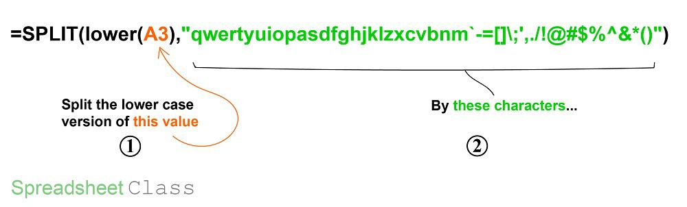
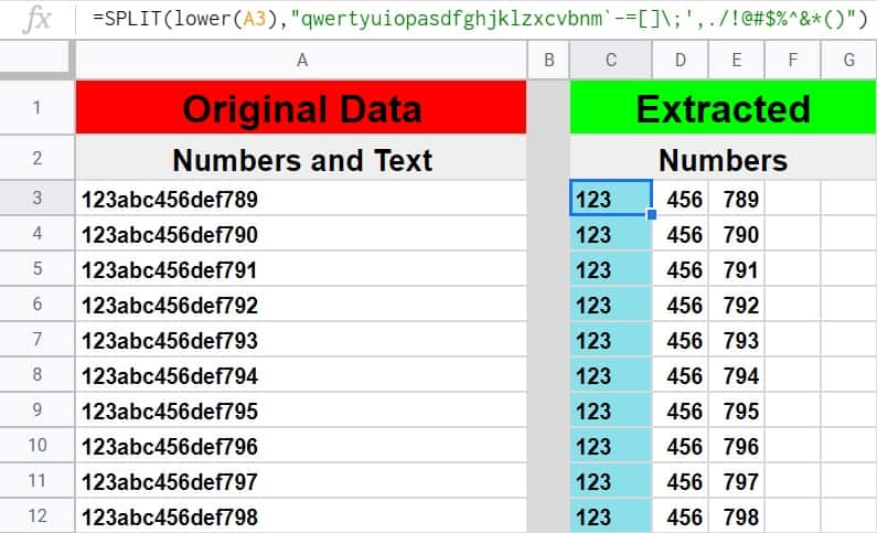
The task: Extract numbers only from a string of text and numbers, and split the consecutive numbers into separate columns

The logic: Split the cells in the range A3:A12, by any text or punctuation character. Wrap the LOWER function around the source range to assure that capital letters are not ignored.

The formula: The formula below, is entered in the blue cells in the range C3:C12, for this example

=SPLIT(lower(A3),”qwertyuiopasdfghjklzxcvbnm`-=[]\;’,./!@#$%^&*()”)

More formulas:

Below are more formulas that perform a similar/exactly the same task as the formula demonstrated in the example above.

Other ways to write the formula in the example above:

=SPLIT(A3,”qwertyuiopasdfghjklzxcvbnmQWERTYUIOPASDFGHJKLZXCVBNM`-=[]\;’,./!@#$%^&*()”)

Extract text into separate columns

Here we are going to use the SPLIT function again as in the example above, but this time we will extract text instead of numbers.

This time there are far fewer characters to be typed into the SPLIT criteria, as there are far fewer digits than there are letters.

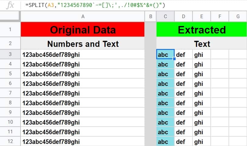
The task: Extract text only from a string of text and numbers, and split the consecutive text characters into separate columns

The logic: Split the cells in the range A3:A12, by any number or punctuation character.

The formula: The formula below, is entered in the blue cells in the range C3:C12, for this example

=SPLIT(A3,”1234567890`-=[]\;’,./!@#$%^&*()”)

Extract N characters starting at the Nth Character

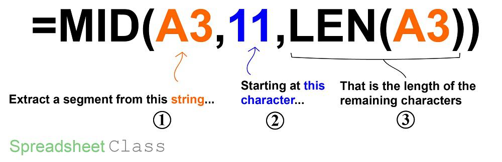
Before we begin extracting full strings of text/numbers etc, let’s go over the MID function.

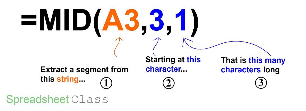
The MID function in Google Sheets will allow you to extract a specified number of characters from a string, starting at a specified character.

The Google Sheets MID function description:

Syntax:
MID(string, starting_at, extract_length)

Formula summary: “Returns a segment of a string.”

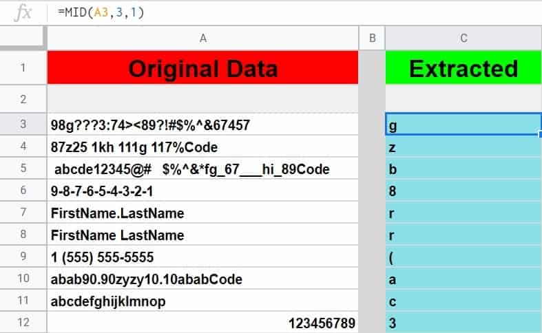
In this example we will extract the third character from a list of character strings. As mentioned above, this is the raw source data that we will be using in every example for the rest of the article.

The task: Extract the third character from each cell/string

The logic: Extract one character, starting at the third character, from the strings in each cell in the range A3:A12

The formula: The formula below, is entered in the blue cells. It is initially into the cell C3, and then copied/filled into the range C3:C12

=MID(A3,3,1)

More formulas:

Below are more formulas that perform a similar/exactly the same task as the formula demonstrated in the example above.

Similar formulas:

• =MID((REGEXREPLACE(A3,”[^[:digit:]]”, “”)),3,1) – Extracts N numbers starting at the Nth number
• =MID((REGEXREPLACE(A3,”[^0-9]”, “”)),3,1) – Extracts N numbers starting at the Nth number
• =MID((REGEXREPLACE(A3,”\D”, “”)),3,1) – Extracts N numbers starting at the Nth number
• =MID((REGEXREPLACE(A3,”[[:digit:]]”, “”)),3,1) – Extracts N non-numbers starting at the Nth non-number
• =MID((REGEXREPLACE(A3,”[0-9]”, “”)),3,1) – Extracts N non-numbers starting at the Nth non-number
• =MID((REGEXREPLACE(A3,”\d”, “”)),3,1) – Extracts N non-numbers starting at the Nth non-number
• =MID((REGEXREPLACE(A3,”[^[:alpha:]]”, “”)),3,1) – Extracts N letters starting at the Nth letter
• =MID((REGEXREPLACE(A3,”[^a-zA-Z]”, “”)),3,1) – Extracts N letters starting at the Nth letter
• =MID((REGEXREPLACE(A3,”[[:alpha:]]”, “”)),3,1) – Extracts N non-letters starting at the Nth non-letter
• =MID((REGEXREPLACE(A3,”[a-zA-Z]”, “”)),3,1) – Extracts N non-letters starting at the Nth non-letter
• =MID((REGEXREPLACE(A3,”[[:alnum:]]”, “”)),3,1) – Extracts N punctuation characters starting at the Nth punctuation character (includes spaces)
• =MID((REGEXREPLACE(A3,”[a-zA-Z0-9]”, “”)),3,1) – Extracts N punctuation characters starting at the Nth punctuation character (includes spaces)
• =MID((REGEXREPLACE(A3,”[^[:punct:]]”, “”)),3,1) – Extracts N punctuation characters starting at the Nth punctuation character (spaces not included)
• =MID((REGEXREPLACE(A3,”[[:word:]]”, “”)),3,1) – Extracts N punctuation characters starting at the Nth punctuation character (spaces included but not underscores)
• =MID((REGEXREPLACE(A3,”\w”, “”)),3,1) – Extracts N punctuation characters starting at the Nth punctuation character (spaces included but not underscores)
• =MID((REGEXREPLACE(A3,”[[:punct:]]”, “”)),3,1) – Extracts N non-punctuation characters starting at the Nth non-punctuation character (includes spaces)
• =MID((REGEXREPLACE(A3,”[^[:alnum:]]”, “”)),3,1) – Extracts N non-punctuation characters starting at the Nth non-punctuation character (spaces not included)
• =MID((REGEXREPLACE(A3,”[^a-zA-Z0-9]”, “”)),3,1) – Extracts N non-punctuation characters starting at the Nth non-punctuation character (spaces not included)
• =MID((REGEXREPLACE(A3,”[^[:word:]]”, “”)),3,1) – Extracts N non-punctuation characters starting at the Nth non-punctuation character (spaces/hyphens not included but underscores are)
• =MID((REGEXREPLACE(A3,”\W”, “”)),3,1) (spaces/hyphens not included but underscores are)

Extract remaining characters starting at Nth character

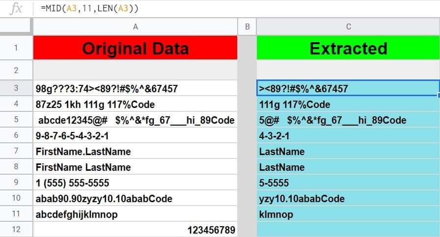
In this example we will use the MID function along with the LEN function, to extract the remaining characters in a string starting at a specified character/position.

Notice that for strings which have less than 11 characters, the formula will output an empty string.

The task: Extract the remaining characters from each cell/string, starting at the 11th character

The logic: Starting at the 11th character, extract the remaining characters from each cell in the range A3:A12

The formula: The formula below, is entered in the blue cells. It is initially into the cell C3, and then copied/filled into the range C3:C12

=MID(A3,11,LEN(A3))

Extract numbers from a string in Google Sheets

Now we will finally begin using the REGEXREPLACE function, to extract whole strings of text, numbers, and other specified character types.

For an in-depth explanation on how to use the REGEXREPLACE and REGEXEXTRACT functions, return to the top of the page for lots of information. But here we will simply use the functions in many different ways.

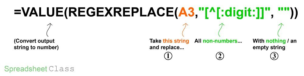
In this example I will show you how to extract numbers from a string in Google Sheets, by replacing any character that is not a number, with nothing/ an empty string.

*In this specific example we are using the VALUE function as well, to assure that the numbers we are extracting are in number format.

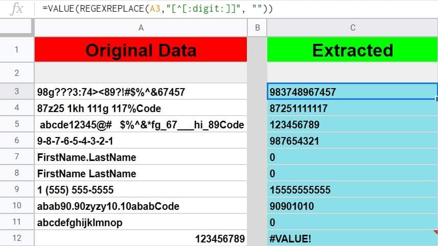
Although we are displaying numbers in our formula output, the formula expects text to be in the input, so notice that in row 12 the formula results in an error because the input for that entry is numbers only… but more specifically is in the number format (hence the right alignment). If this same exact string (123456789) were simply changed to plain text format, the formula would output the entire string.

The task: Extract the numbers from each cell/string

The logic: Extract the numbers from each cell in the range A3:A12, by replacing any non-digit with an empty string

The formula: The formula below, is entered in the blue cells. It is initially into the cell C3, and then copied/filled into the range C3:C12

=VALUE(REGEXREPLACE(A3,”[^[:digit:]]”, “”))

More formulas:

Below are more formulas that perform a similar/exactly the same task as the formula demonstrated in the example above.

Other ways to write the formula in the example above:

• =VALUE(REGEXREPLACE(A3,”[^0-9]”, “”))
• =VALUE(REGEXREPLACE(A3,”\D”, “”))

Similar formulas:

• =REGEXEXTRACT (A3, “(\d+\.?\d+)”) – Extracts numbers with decimal
• =REGEXREPLACE(A3,”[[:digit:]]”, “”) – Extracts non-numbers
• =REGEXREPLACE(A3,”[0-9]”, “”) – Extracts non-numbers
• =REGEXREPLACE(A3,”\d”, “”) – Extracts non-numbers

Extract text from a string in Google Sheets

Now that you know how to extract numbers by using the REGEXREPLACE function, a simple change in the character class / regular expression will now allow us to extract all different types of characters.

In this example, I’ll show you how to extract text from a string in Google Sheets.

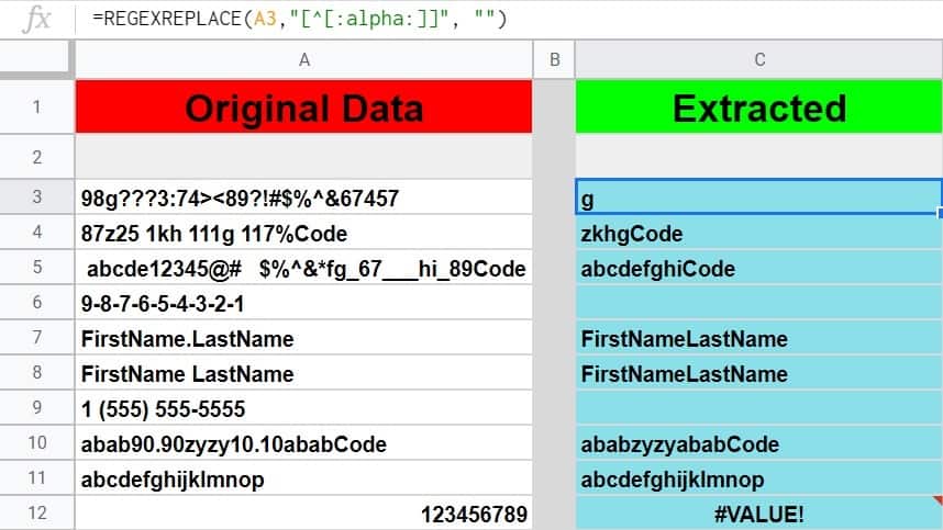
Notice that when using this formula on strings that contain no text, the formula will output an empty string.

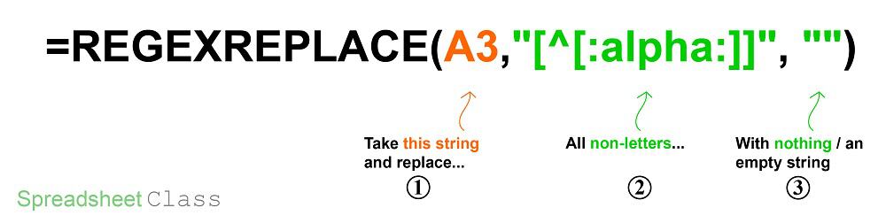
The task: Extract the text from each cell/string

The logic: Extract the text from each cell in the range A3:A12, by replacing any non-text character with an empty string

The formula: The formula below, is entered in the blue cells. It is initially into the cell C3, and then copied/filled into the range C3:C12

=REGEXREPLACE(A3,”[^[:alpha:]]”, “”)

More formulas:

Below are more formulas that perform a similar/exactly the same task as the formula demonstrated in the example above.

Other ways to write the formula in the example above:

• =REGEXREPLACE(A3,”[^a-zA-Z]”, “”)

Similar formulas:

• =REGEXREPLACE(A3,”[[:alpha:]]”, “”) – Extracts non-text characters
• =REGEXREPLACE(A3,”[a-zA-Z]”, “”) – Extracts non-text characters

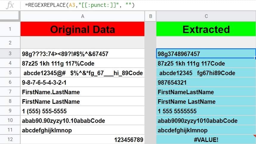
How to remove punctuation from a string in Google Sheets

Now I am going to show you how to remove punctuation from strings in Google Sheets, or in other words how to extract non-punctuation characters.

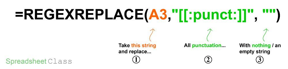
The task: Remove the punctuation from each cell/string

The logic: Remove the punctuation from each cell in the range A3:A12, by replacing any non-punctuation character with an empty string

The formula: The formula below, is entered in the blue cells. It is initially into the cell C3, and then copied/filled into the range C3:C12

=REGEXREPLACE(A3,”[[:punct:]]”, “”)

More formulas:

Below are more formulas that perform a similar/exactly the same task as the formula demonstrated in the example above.

Similar formulas:

• =REGEXREPLACE(A3,”[^[:alnum:]]”, “”) – Removes punctuation (and spaces)
• =REGEXREPLACE(A3,”[^a-zA-Z0-9]”, “”) – Removes punctuation (and spaces)
• =REGEXREPLACE(A3,”[^[:word:]]”, “”) – Removes punctuation (and spaces, but not underscores)
• =REGEXREPLACE(A3,”\W”, “”) – Removes punctuation (and spaces, but not underscores)
• =REGEXREPLACE(A3,”[[:alnum:]]”, “”) – Extracts punctuation (spaces included)
• =REGEXREPLACE(A3,”[a-zA-Z0-9]”, “”) – Extracts punctuation (spaces included)
• =REGEXREPLACE(A3,”[^[:punct:]]”, “”) – Extracts punctuation (spaces not included)
• =REGEXREPLACE(A3,”[[:word:]]”, “”) – Extracts punctuation (spaces included but not underscores)
• =REGEXREPLACE(A3,”\w”, “”) – Extracts punctuation (spaces included but not underscores)

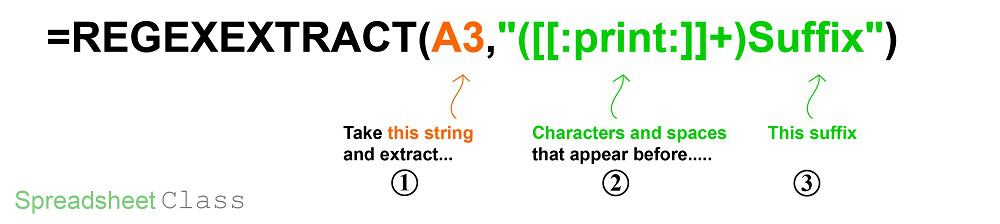
Extract characters before a suffix- Part 1

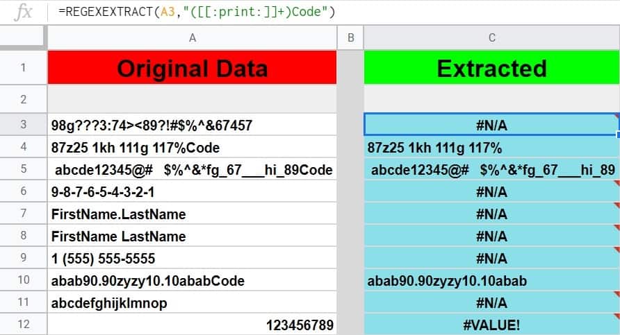
In this example I will show you how to extract the characters that are found before a suffix. Since we are using the same assortment of source data in each example, note that not all strings contain the suffix that we are searching for in this example.

Note that rows 4, 5, and 10 are the only entries/rows that contain the suffix “Code”, and so this is why this particular formula will only work on these entries.

The task: Extract the characters before a suffix, from each cell/string

The logic: Extract a string of characters before the suffix “Code”, from each cell in the range A3:A12, by specifying a suffix after the character class, in the REGEXEXTRACT regular expression

The formula: The formula below, is entered in the blue cells. It is initially into the cell C3, and then copied/filled into the range C3:C12

=REGEXEXTRACT(A3,”([[:print:]]+)Code”)

More formulas:

Below are more formulas that perform a similar/exactly the same task as the formula demonstrated in the example above.

Similar formulas:

• =REGEXEXTRACT(A3,”([[:graph:]]+)Code”) – Extracts characters before a suffix (spaces not included)

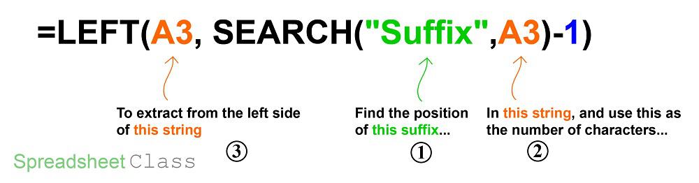
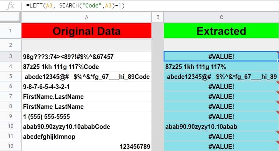
Extract characters before a suffix- Part 2

Another way to extract characters before a suffix is by using the LEFT and SEARCH function.

Just like in the last example, only the entries/rows that actually contain the suffix “Code” can be used with this formula.

The task: Extract the characters that are found before a specified suffix, from each cell/string

The logic: Extract a string of characters before the suffix “Code”, from each cell in the range A3:A12, by using the SEARCH function to locate the position of a suffix and therefore provide the number of characters to extract with the LEFT function.

The formula: The formula below, is entered in the blue cells. It is initially into the cell C3, and then copied/filled into the range C3:C12

=LEFT(A3, SEARCH(“Code”,A3)-1)

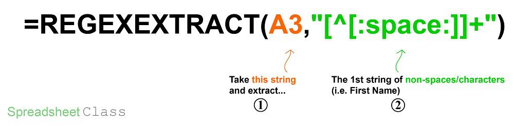
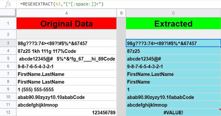
Extract the first word from a cell- Part 1

You may find situations where you need to extract the first name/word from a cell Google Sheets, and so here I’ll show you how to do this by using the REGEXEXTRACT function.

The task: Extract the first name from each cell/string

The logic: Extract the first word/name (1st string of characters before a space), from each cell in the range A3:A12, by extracting a string of non-space characters found before the first space

The formula: The formula below, is entered in the blue cells. It is initially into the cell C3, and then copied/filled into the range C3:C12

=REGEXEXTRACT(A3,”[^[:space:]]+”)

More formulas:

Below are more formulas that perform a similar/exactly the same task as the formula demonstrated in the example above.

Other ways to write the formula in the example above:

• =REGEXEXTRACT(A3,”\S+”)
• =REGEXEXTRACT(A3,”[[:graph:]]+”)

Similar formulas:

• =REGEXEXTRACT(A3,”[[:digit:]]+”) – Extracts first number string
• =REGEXEXTRACT(A3,”[0-9]+”) – Extracts first number string
• =REGEXEXTRACT(A3,”\d+”) – Extracts first number string
• =REGEXEXTRACT(A3,”[^[:digit:]]+”) – Extracts first non-number string
• =REGEXEXTRACT(A3,”[^0-9]+”) – Extracts first non-number string
• =REGEXEXTRACT(A3,”\D+”) – Extracts first non-number string
• =REGEXEXTRACT(A3,”[[:alpha:]]+”) – Extracts first text string
• =REGEXEXTRACT(A3,”[a-zA-Z]+”) – Extracts first text string
• =REGEXEXTRACT(A3,”[^[:alpha:]]+”) – Extracts first non-text string
• =REGEXEXTRACT(A3,”[^a-zA-Z]+”) – Extracts first non-text string
• =REGEXEXTRACT(A3,”[[:alnum:]]+”) – Extracts first non-punctuation string (spaces not included)
• =REGEXEXTRACT(A3,”[a-zA-Z0-9]+”) – Extracts first non-punctuation string (spaces not included)
• =REGEXEXTRACT(A3,”[^[:punct:]]+”) – Extracts first non-punctuation string (spaces included)
• =REGEXEXTRACT(A3,”[[:word:]]+”) – Extracts first non-punctuation string (spaces/hyphens not included but underscores are)
• =REGEXEXTRACT(A3,”\w+”) – Extracts first non-punctuation string (spaces/hyphens not included but underscores are)
• =REGEXEXTRACT(A3,”[^[:alnum:]]+”) – Extracts first punctuation string (spaces included)
• =REGEXEXTRACT(A3,”[^a-zA-Z0-9]+”) – Extracts first punctuation string (spaces included)
• =REGEXEXTRACT(A3,”[[:punct:]]+”)- Extracts first punctuation string (spaces not included)
• =REGEXEXTRACT(A3,”[^[:word:]]”)- Extracts first punctuation string (underscores not included)
• =REGEXEXTRACT(A3,”\W+”)- Extracts first punctuation string (underscores not included)

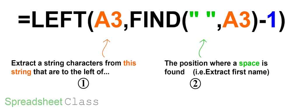
Extract first name/word- Part 2

In this example I will show you another way to extract the first name/word in Google Sheets, by using the LEFT and FIND functions. This will show you the first string of characters that appear before the first space.

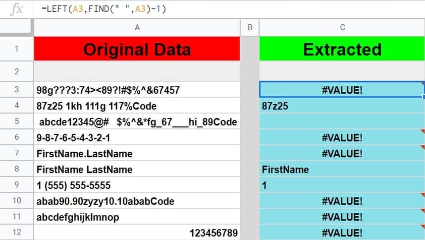
Notice that this formula will only work on strings that have a space within them. Also notice that in row 5 where the space is the first character/position within a string, the formula outputs an empty string.

The task: Extract the first word from each cell/string

The logic: Extract the first word (i.e. name) from each cell in the range A3:A12, by using the FIND function to provide the criteria for the LEFT function

The formula: The formula below, is entered in the blue cells. It is initially into the cell C3, and then copied/filled into the range C3:C12

=LEFT(A3,FIND(” “,A3)-1)

Extract the first character from a string

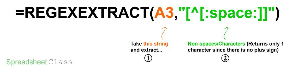
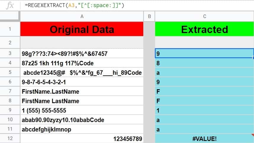
In this example I will show you how to extract the first character from a string in Google Sheets. You will notice that this formula is almost identical to a formula that was used previously in the article to extract first name… but note that in this example there is no plus sign used in the character class, which means that only a single character will be extracted by the REGEXEXTRACT function.

The task: Extract the first character from each cell/string

The logic: Extract the first character from each cell in the range A3:A12, by extracting the first non-space character with the REGEXEXTRACT function (without using a plus sign on the character class)

The formula: The formula below, is entered in the blue cells. It is initially into the cell C3, and then copied/filled into the range C3:C12

=REGEXEXTRACT(A3,”[^[:space:]]”)

More formulas:

Below are more formulas that perform a similar/exactly the same task as the formula demonstrated in the example above.

Other ways to write the formula in the example above:

=REGEXEXTRACT(A3,”[[:graph:]]”)

=REGEXEXTRACT(A3,”\S”)

Similar formulas:

=REGEXEXTRACT(A3,”[[:print:]]”) – Extracts first character (spaces included)

Extract last name from a cell

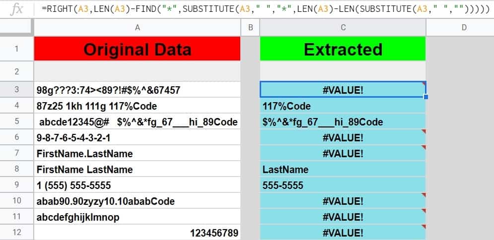
In this example, I will show you a formula that you can use to extract last name from a cell in Google Sheets.

Notice that this formula will only work on strings/entries that contain a space within them.

The task: Extract the last name from each cell/string

The logic: Extract the last name from each cell in the range A3:A12, by using the following functions: RIGHT, LEN, FIND, and SUBSTITUTE.

The formula: The formula below, is entered in the blue cells. It is initially into the cell C3, and then copied/filled into the range C3:C12

=RIGHT(A3,LEN(A3)-FIND(“*”,SUBSTITUTE(A3,” “,”*”,LEN(A3)-LEN(SUBSTITUTE(A3,” “,””)))))

Extract Nth word in Google Sheets

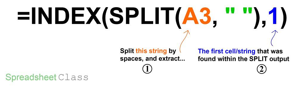
So we have already went over formulas that extract the first or last word from a cell… but if you want to specify the word you would like to extract in Google Sheets you can do this by using the INDEX and SPLIT functions.

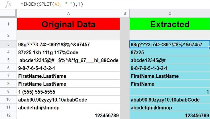
Notice that for strings that have no space within them, this formula will extract the entire contents of the cell. Also notice that with this formula, in row 5 that even though a space is in the first position of the string… the first word/string of actual characters is still found and displayed (where in a previous example this leading space caused a different formula to output an empty string).

The task: Extract the first word from each cell/string

The logic: Extract the first word from each cell in the range A3:A12, by splitting the string(s) by a space, and extracting the first cell from the split results.

The formula: The formula below, is entered in the blue cells. It is initially into the cell C3, and then copied/filled into the range C3:C12

=INDEX(SPLIT(A3, ” “),1)

LEFT function / RIGHT function: Extract N Characters from the left/right of a string

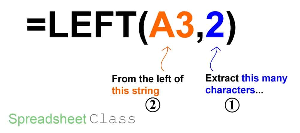
In this example, we will extract a specified number of characters from the left side of a string, by using the LEFT function.

The LEFT function in Google Sheets will display a substring that is a specified number of characters long, starting at the beginning of a string that you specify.

The Google Sheets LEFT function description:

Syntax:
LEFT(string, [number_of_characters])

Formula summary: “Returns a substring from the beginning of a specified string.”

The Google Sheets RIGHT function description:

Syntax:
RIGHT(string, [number_of_characters])

Formula summary: “Returns a substring from the end of a specified string.”

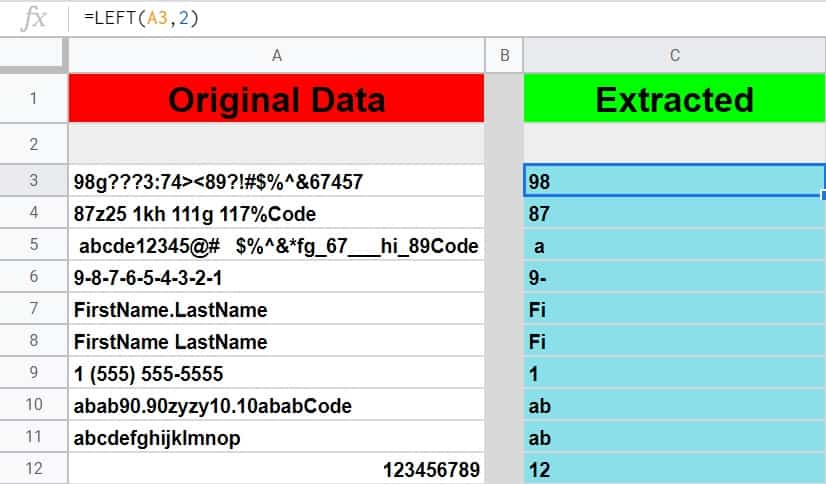
The task: Extract 2 characters from the left side of each cell/string

The logic: Extract 2 characters from the left of each cell in the range A3:A12, by using the LEFT function

The formula: The formula below, is entered in the blue cells. It is initially into the cell C3, and then copied/filled into the range C3:C12

=LEFT(A3,2)

More formulas:

Below are more formulas that perform a similar/exactly the same task as the formula demonstrated in the example above.

Similar formulas:

• =RIGHT(A3,2) – Extracts N characters to the right of a string
• =LEFT(REGEXREPLACE(A3,”\D+”, “”),2)) – Extracts N numbers to the left of a string
• =RIGHT(REGEXREPLACE(A3,”\D+”, “”),2)) – Extracts N numbers to the right of a string
• =LEFT(REGEXREPLACE(A3,”\d+”, “”),2)) – Extracts N letters to the left of a string
• =RIGHT(REGEXREPLACE(A3,”\d+”, “”),2)) – Extracts N letters to the right of a string

REPLACE & SUBSTITUTE

Now let’s go over the REPLACE function, and the SUBSTITUTE function, which are both formulas the replace text, with specified text. But the replace function identifies the text to be replaced by referring to the position of the text, where the SUBSTITUTE function iedentifies the text to be replaced by specifying the string of text to be replaced.

REPLACE function: Replace part of a text string with a different text string

The REPLACE function replaces part of a text string with a different text string (identifies text to replace by specifying position)

In this example we have a string of numbers and text (a code), and we want to replace the letters “abc” with capital letters, like this “ABC”. We will use the REPLACE function to do this and then in the next example we will use another function to do the same thing.

With the REPLACE function, first we specify the cell that we want to replace text in, type a comma, type the number that represents the position of the first character that you want to replace, type a comma, then type a number that represents how many characters you want to replace, type a comma, then between quotation marks type the string of text / characters that you want to replace the characters you specified.

The Google Sheets REPLACE function description:

Syntax:
REPLACE(text, position, length, new_text)

Formula summary: “Replaces part of a text string with a different text string.”

The task: Replace the letter “abc” with the letters “ABC”

The logic: Use the REPLACE function to replace 3 characters, starting at the 4th character, where the replacement text is “ABC”

The formula: The formula below, is entered in the blue cells. It is initially into the cell C3, and then copied/filled into the range C3:C11

=REPLACE(A3,4,3,”ABC”)

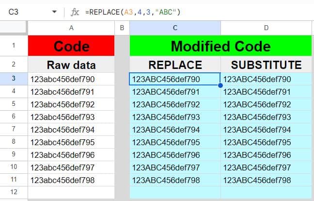
As you can see in the image above, the string “abc” has been replaced with the string “ABC”, in each code / each row.

Note that for this example, the same REPLACE function worked in each row because the characters to be replaced were the same length / in the same postion for every row, but the formula in the next example would be able to handle this task even if the characters to be replaced were not in the same position each time.

SUBSTITUTE function: Replace existing text with new text in a string

Now let’s go over how to use the SUBSTITUTE function, to perform the same task as in the last example (replace “Abc” with “ABC”)

The SUBSTITUTE function replaces a string of specified text / characters, with another strong of specified text / characters… so unlike the REPLACE function, you do not have to specify the position / length.

With the SUBSTITUTE function, first we specify the cell that we want to replace text in, type a comma, between quotation marks type the string of characters that you want to replace, type a comma, then between quotation marks type the string of text / characters that you want to replace the characters you specified.

The Google Sheets SUBSTITUTE function description:

Syntax:
SUBSTITUTE(text_to_search, search_for, replace_with, [occurrence_number])

Formula summary: “Replaces existing text with new text in a string.”

The task: Replace the letter “abc” with the letters “ABC”

The logic: Use the SUBSTITUTE function to replace the characters “abc”, with the characters “ABC”

The formula: The formula below, is entered in the blue cells. It is initially into the cell C3, and then copied/filled into the range C3:C11

=SUBSTITUTE(A3,”abc”,”ABC”)

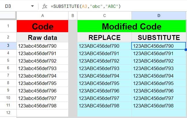
Notice in the image above, the same result was achieved from the last example, where the characters “abc” were replaced with the characters “ABC”. But this time we used the SUBSTITUTE function to do it.

Lesson review

Let’s summarize the main formulas that we went over in this lesson.

The formulas for extracting in Google Sheets:

Extract numbers into separate columns

• =SPLIT(lower(A3),”qwertyuiopasdfghjklzxcvbnm`-=[]\;’,./!@#$%^&*()”)

Extract text into separate columns

• =SPLIT(A3,”1234567890`-=[]\;’,./!@#$%^&*()”)

Extract N characters starting at the Nth Character

• =MID(A3,3,1)

Extract remaining characters starting at Nth character

• =MID(A3,11,LEN(A3))

Extract numbers from a string

• =VALUE(REGEXREPLACE(A3,”[^[:digit:]]”, “”))

Extract text from a string

• =REGEXREPLACE(A3,”[^[:alpha:]]”, “”)

Remove punctuation

• =REGEXREPLACE(A3,”[[:punct:]]”, “”)

Extract characters before a suffix

• =REGEXEXTRACT(A3,”([[:print:]]+)Code”)
• =LEFT(A3, SEARCH(“Code”,A3)-1)

Extract first word / name

• =REGEXEXTRACT(A3,”[^[:space:]]+”)
• =LEFT(A3,FIND(” “,A3)-1)

Extract first character

• =REGEXEXTRACT(A3,“[^[:space:]]”)

Extract last name

• =RIGHT(A3,LEN(A3)-FIND(“*”,SUBSTITUTE(A3,” “,”*”,LEN(A3)-LEN(SUBSTITUTE(A3,” “,””)))))

Extract Nth word

• =INDEX(SPLIT(A3, ” “),1)

Extract N characters from the left / right

• =LEFT(A3,2)

Replace part of a text string with a different text string (identifies text to replace by specifying position)

• =REPLACE(A3,4,3,”ABC”)

Replace existing text with new text in a string (identifies text to replace by specifying string)

• =SUBSTITUTE(A3,”abc”,”ABC”)

Pop Quiz: Test your knowledge

Answer the questions below about extracting, to refine your knowledge! Scroll to the very bottom to find the answers to the quiz.

Classroom downloads:

Click here to get your Google Sheets cheat sheet

Or click here to take the dashboards course

Extraction formulas cheat sheet (PDF)

Question #1

Which of the following formulas will extract text?

1. =VALUE(REGEXREPLACE(A1,”[^[:digit:]]”, “”))
2. =REGEXREPLACE(C1,”[^[:alpha:]]”, “”)
3. =REGEXREPLACE(G1,”[[:punct:]]”, “”)

Question #2

Which of the following formulas will extract numbers?

1. =REGEXREPLACE(Z11,”[[:punct:]]”, “”)
2. =REGEXREPLACE(J7,”[^[:alpha:]]”, “”)
3. =VALUE(REGEXREPLACE(P17,”[^[:digit:]]”, “”))

Question #3

True or False: The REGEXREPLACE function can be used to extract/replace EVERY instance of a specified character type, where the REGEXEXTRACT function can be used to extract parts “substrings” from the source string.

1. True
2. False

Question #4

Which of the following character classes represents “non-text characters”?

1. [^[:alpha:]]  ~  [^a-zA-Z]
2. [[:alpha:]]  ~  [a-zA-Z]

Question #5

Which of the following character classes CONTAIN visible characters (Select all that apply)?

1. [[:graph:]]
2. [^[:graph:]]
3. [[:space:]] ~   \s
4. [^[:space:]]  ~   \S
5. [[:print:]]
6. [^[:print:]]

Answers to the questions above:

Question 1: 2

Question 2: 3

Question 3: 1

Question 4: 1

Question 5: 1, 4, 5