

The data organizer template for Google Sheets is a unique and incredibly useful tool that will help you create clean reports and make quick calculations, for spreadsheet data in almost any industry.
With this report generator you will be able to quickly organize / analyze your data, and build professional reports without having to use any formulas.
Simply import your data, then set your preferences in the template, and the spreadsheet will do the rest for you!
Read below to learn how to use this template. Note that some tabs / cells in the template are locked and will display a warning if you try to edit them. Below I will tell you which places in the template are meant to be edited.
Get the report builder template
How to use the report builder
The report builder breaks down into 5 main parts / steps:
- Import your data
- Basic Report: Select the columns that you want to use
- Calculated Report: Organize and calculate the data
- Apply color coding
- Clean Report: View / download the report
Importing your data
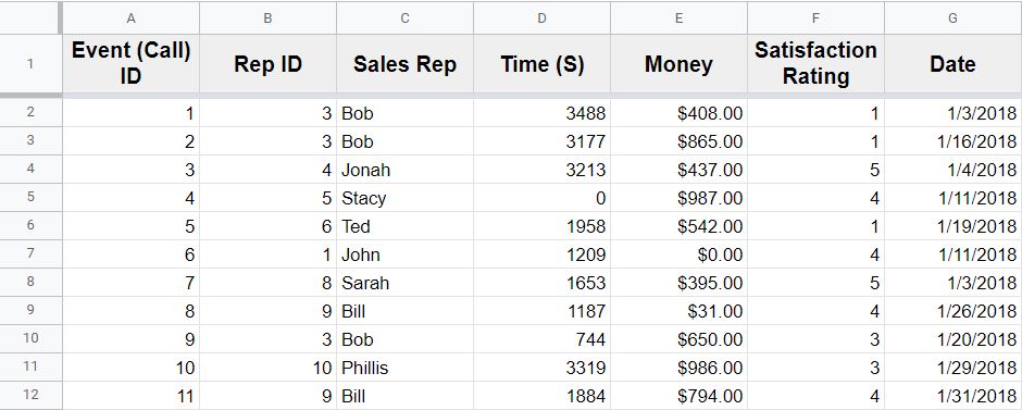
The first step is to import your data into the “Data Import” tab.
Any cell in this tab can be edited.
Click here to learn how to import CSV data into a Google spreadsheet.
Note that this report builder is intended for reports that only have 1 header row. If you have a report that you want to use with this template that has more than one header, feel free to email me and I’ll be happy to help you.
Choose your columns (Basic Report)
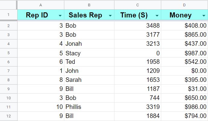
The next step in the process is to select the columns that you want to be in your final report. Raw reports often come with more columns than you need, and so this will allow you to narrow down your report to only the essential columns.
On the “Basic Report” tab, simply click the drop down menus in row 1 to choose the name of the columns that you want to view, and the data for each selected header / column name will instantly appear below.
You can edit row 1 (blue cells) of this tab.
You can select the columns in any order that you want, and can even select the same column more than once if you want to.
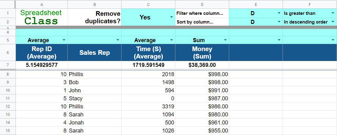
Organize and calculate the data (Calculated Report)
The “Calculated Report” tab is probably the coolest tab in the template. Here you can sort your data, filter it, remove duplicates, calculate totals and averages, count non-blank cells, count unique cells, and count cells that meet a specified criteria.
The blue cells (detailed below) can be edited in this tab.
Remove duplicates
First, use cell C1 to indicate whether or not you want duplicate rows to be removed from the report. If there are no duplicate rows, this selection will have no effect.
Click here to learn more about removing duplicates in Google Sheets.
Filter the data
Next, you can filter your data based on custom criteria.
Click here to learn more about filtering data in Google Sheets.
Choose the criteria column
In cell E1, select the criteria column (The column that contains the “criteria” for filtering). For example if you wanted to filter a report, and show only the rows where revenue earned was more than 0 dollars, the criteria column would be the column that contains the revenue earned.
Select the appropriate operator
Then in cell F1, choose from the following options / operators:
- Is equal to
- Is not equal to
- Is greater than
- Is less than
- Is greater than or equal to
- Is less than or equal to
The selection of this operator will determine how the sheet interacts with the criteria that you set in the next step.
Enter the filter criteria
Then in cell H1, enter the criteria itself for the filter. For example, if you wanted to filter your report so that only the rows pertaining to the sales representative “Bob” are displayed, then you would enter the text “Bob” in cell H1. Or using the revenue example mentioned above, you would enter the number “0” in cell H1.
Sort the data
Next, you can choose to sort your data by the column of your choice, in the order of your choice.
Click here to learn more about sorting data in Google Sheets.
Choose the column to sort by
In cell E2, choose the column that you want to sort your data by
Choose the order to sort in
In cell F2, choose from the following options:
- In ascending order
- In descending order
Performing calculations
Next, you can choose from a variety of calculations to perform on each column of your data.
Click here to learn more about using formulas in Google Sheets.
Or, click here to download your free Google Sheets formulas cheat sheet.
In row 5 of the “Calculated Report” tab, you can select from the types of calculations listed below, by using a drop down menu.
In row 4, you can enter the criteria for the “Count if equal to” calculation type.
Sum
Choose this option to sum / add up all of the values in a column.
Average
Choose this option to average all of the values in a column
Count if not blank
Choose this option to count all of the cells in a column that are not blank (i.e. count the number of entries / rows containing data)
Count unique cells
This option will count the number of unique values in a column, or in other words will count how many different types of values are found in the column.
Count if cells are equal to criteria
This option will allow you to count the number of times that a specified value (Text / Number, etc.) is found in a column. When this option is chosen, you can specify the value that you are counting, in row 4.
For example, if you wanted to count the number of times that the name “Bob” appears in a certain column, you would enter the name “Bob” in row 4.
Apply color coding
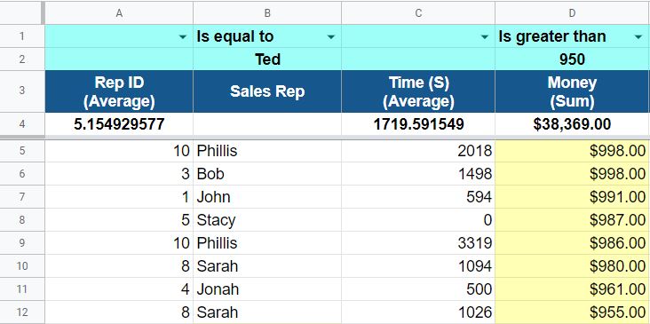
Next, you can choose to apply color coding (Conditional Formatting) to your data.
In the “Color Coding” tab, you can specify criteria in each column that will make the cells turn yellow if they meet your criteria.
For example, if you wanted to highlight all of the cells in column D that contain a value of greater than 950, you would do the following:
- In cell D1, select “Is greater than”.
- In cell D2, enter the number “950”
Select the correct operator in row 1
Select the appropriate operator from row 1, in the column that you want to apply color coding to, by selecting from one of these options:
- Is equal to
- Is not equal to
- Is greater than
- Is less than
- Is greater than or equal to
- Is less than or equal to
This selection will affect how the conditional formatting interacts with the criteria that you set below.
Enter the criteria in row 2
In row 2, enter the criteria that you want to be color coded, in the column(s) of your choice.
This template / content was created by Corey Bustos / SpreadsheetClass.com
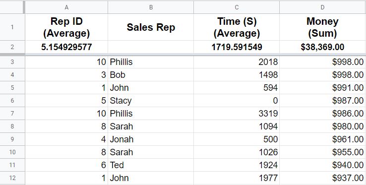
View / download the “Clean report”
The final tab in this template will allow you to view a clean / plain report, showing your chosen columns and the calculations that were applied in the previous steps.
You can choose to simply view this tab, or you can also download / export this tab into a CSV file.
Click here to learn how to export CSV data from a Google spreadsheet.
The link to the Google Sheets report builder template can be found near the top of this page. I hope that you enjoy this template, and that it makes your job easier!