

When using formulas in Microsoft Excel you will often need to apply a formula to an entire column, and this can be done quite easily by using array formulas.
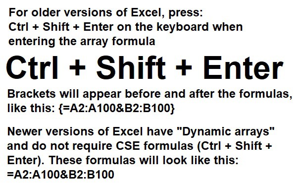
To apply a formula to an entire column in Excel by using a single formula, change the single cell references in your formula into references that refer to a column or range of cells. In older versions of Excel, press Ctrl + Shift + Enter on the keyboard when entering the formula (Brackets will appear before and after the formula).
For example, note the two IF formulas below. The first one is an ordinary IF formula that refers to a single cell, but the second formula uses an "array", and is applied to multiple cells.
=IF(A1=1,1,0)
=IF(A1:A100=1,1,0)
Ctrl + Shift + Enter Version (For older Excel Versions):
{=IF(A1:A100=1,1,0)}
This article shows how to use array formulas in Excel, but click here if you want to learn how to use arrays / ARRAYFORMULA in Google Sheets.
Dynamic arrays vs. CSE (Ctrl + Shift + Enter) formulas
In newer versions of Excel, you can simply change the cell references into range references, and the formula will apply to multiple cells / the entire range. These newer versions do this by using "dynamic arrays".
An example of a dynamic array formula looks like this: =A1:A100
But in older versions, when you would normally press "Enter" to enter your formula into the cell, when using an array, you will need to hold "Ctrl" and "Shift" on the keyboard, and then press "Enter", to insert the array formula. After doing this, brackets will appear at the beginning and end of your formula, or in other words your formula will be wrapped in brackets.
An example of a CSE formula looks like this: {=A1:A100}
Note that some newer versions of Excel, such as Excel online, will not allow you to use CSE formulas, which is okay because you do not need them.
Here are the various ways to use array formulas:
Refer to a column
- =A2:A1001
- {=A2:A1001}
Refer to a row
- =B1:V1
- {=B1:V1}
Sum / Multiply columns
- =A3:A1001+B3:B1001
- {=A3:A1001+B3:B1001}
- =A3:A1001*B3:B1001
- {=A3:A1001*B3:B1001}
IF function with an array
- =IF(B3:B1001>0.6,"Passing","Fail")
- {=IF(B3:B1001>0.6,"Passing","Fail")}
Combine first and last name
- =B3:B1001&", "&A3:A1001
- {=B3:B1001&", "&A3:A1001}
Sum entire tables of data
- =A3:B1001+D3:E1001+G3:H1001
- {=A3:B1001+D3:E1001+G3:H1001}
Pulling data from another sheet
- =List!A3:B1001
- {=List!A3:B1001}
This article focuses specifically on using array formulas to apply formulas to columns and other ranges. But if you are wanting to know how to copy formulas quickly down a column so that there are formulas in each cell, read this article on using “fill down” to copy formulas, which uses some of the same example data that you will find in this article. This is done to show you a different method/formula for achieving the same tasks.
Referring to a column with an array formula
One of the most common and basic ways to use an array formula, is all by itself without another formula being involved… to simply refer to a column or range of data with a single formula.
This is how we will use an array to begin with, but then after you get a good grasp on using the formula itself, we will move on to using arrays to apply other formulas across ranges of cells.
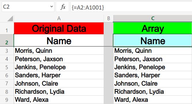
So in this example we will display a list of names from one column, in another column in the spreadsheet.
The task: Display a list of names in another column
The logic: In column C, refer to the list of names that are in column A with an array formula
The formula: The formula below, is entered in the blue cell (C2), for this example
=A2:A1001
{=A2:A1001}
Referring to a row with an array formula
It’s good to note that you can also use arrays to refer to rows / horizontal ranges as well.
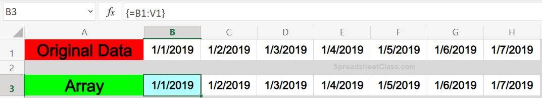
In this example we will refer to a row of cells that have dates in them, and display that list of dates in another row by using an array formula.
The task: Display a list of dates in another row
The logic: In row 3, refer to the list of dates that are in row 1 with an array formula
The formula: The formula below, is entered in the blue cell (B3), for this example
=B1:V1
{=B1:V1}
By SpreadsheetClass.com
How to SUM and multiply columns in Excel
Now let's use an array formula to extend a formula in Excel, so that it applies to an entire column.
You may often find the need to sum or multiply entire columns in Excel, and if you want to achieve this with a single formula then using an array is the way to do it.
This example shows how to use an array formula to extend addition and multiplication formulas.
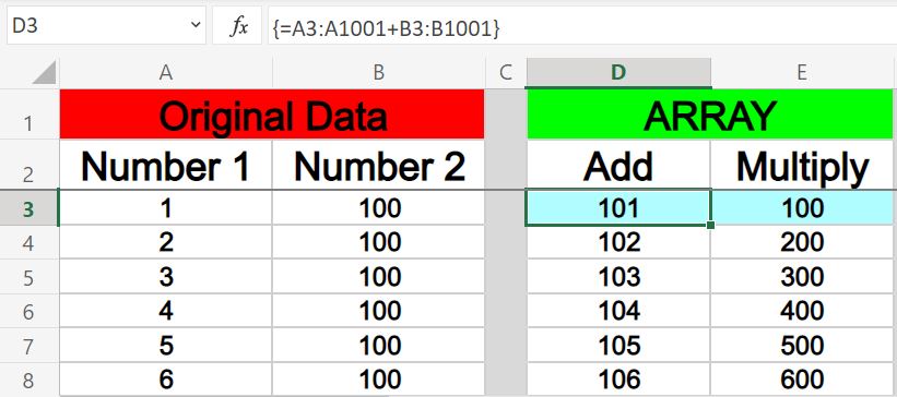
Columns A and B are lists of numbers… and columns D and E add/multiply these numbers by extending addition and multiplication formulas down the column with an array.
In column D, you can see that the addition formula in cell D3 extends its functionality downward into the cells below by using only a single formula, and you can see in column E that the multiplication formula does the same.
The task: Apply the addition and multiplication formulas to an entire column
The logic: Turn the addition and multiplication formulas into an array formula, and specify an entire column as the range
Formula: The formulas below are entered initially into cells D3 and E3 (blue cells), for this example
=A3:A1001+B3:B1001 (Entered in cell D3)
{=A3:A1001+B3:B1001}
=A3:A1001*B3:B1001 (Entered in cell E3)
{=A3:A1001*B3:B1001}
Using an array to extend the IF function
Here is another example where we will apply a formula to an entire column in Excel, but this time we will use the IF function.
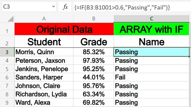
Let's say that you have an IF formula that you have setup to display whether a student is passing/failing based on their grade, and that you want to apply this formula to the entire column. We will do this by turning the IF formula into an array formula.
In the example image below, in columns A and B, is a list of student names and their grades. The formula in column C uses the IF function to display "Passing" if the student's grade is above 60% (0.6), and displays "Fail" if the grade is not above 60%. But the most important thing to note in this example, is that the IF function has been applied to the column by using an array formula.
The task: Apply the IF formula to an entire column
The logic: Turn the IF formula into an array formula, and specify an entire column as the range
The formula: The formula below, is entered in the blue cell (C3), for this example
=IF(B3:B1001>0.6,"Passing","Fail")
{=IF(B3:B1001>0.6,"Passing","Fail")}
How to combine first and last name with an array formula
Another very useful way that you can use an array, is to combine columns, such as when you need to combine first and last name into a single column.
When using an array formula to combine cells/columns, you must use the "&" operator between each of the values/references that you specify (shown in the example).
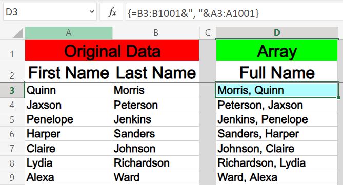
In the example image below, column A has first names and column B has last names.
By using an array formula function with the "&" operator, these names are combined in column D.
The task: Combine the first and last names into "Last, First" format
The logic: Horizontally combine columns A and B, with a comma and a space between them, by using an array formula and the "&" operator
The formula: The formula below, is entered in the blue cell (D3), for this example
=B3:B1001&", "&A3:A1001
{=B3:B1001&", "&A3:A1001}
How to sum entire tables of data with an array formula
Earlier I showed you how to sum columns of data with an array formula, but you can also use this function to sum data across entire tables of data.
When you add a range that has two or more columns/rows to another range of the same size, the array will sum each row/column across the ranges specified.
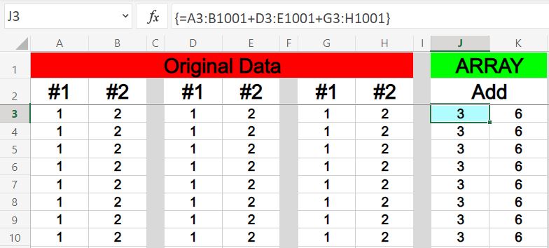
So as you'll see in the formula below, there are three different two-column tables that are being added together with the array formula. The first column of the first range is added to the first column of the second range and then added to the first column of the third range. The function does the same for the second column as well, or for any number of columns as long as the range you are adding are the same size.
This can be visualized as stacking the tables on top of each other and then summing the stacked/overlapping numbers.
The task: Sum the values from three different tables, where each column from each table is added to the same column from the other tables
The logic: Use an array formula to sum the columns from three different two-column ranges, where the first columns are added with the other first columns, and the second columns are added with the other second columns
The formula: The formula below, is entered in the blue cell (J3), for this example
=A3:B1001+D3:E1001+G3:H1001
{=A3:B1001+D3:E1001+G3:H1001}
This content was originally created and written by SpreadsheetClass.com
Pull data from another sheet with array formula
A very common situation that requires the use of an array formula, is when you need to pull data from another sheet (tab) in Excel. Earlier we went over how to simply refer to a range of data by using an array within the same tab, and you can use this same method to refer to data in another tab as long as you specify the tab name that you are pulling the data from, when typing the reference into the formula.
In this example we will cover two important things. The first, is that you can use an array formula to refer to data on other tabs, and the second is that you can use an array formula to refer to the entire range of data with multiple rows and columns.
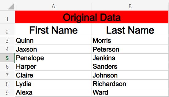
In this example we have a list of first and last names on one tab, that we want to display in another tab. To do this follow the example below.
As with most formulas, when using an array to refer to data from another tab, type the name of the tab that you are pulling from, followed by an exclamation point, followed by the row/column reference.
Remember that if your tab name has a space in it, you must type apostrophes before and after the tab name (Example: 'Tab Name'!A3:B). However in this example the tab name that we will use is named "List", and so we don't need apostrophes.
The task: Display the data that is in columns A and B from the tab that is named "List", in columns A and B in a new/different tab
The logic: In a new tab, display the data from columns A and B from the "List" tab, by referring to the data with an array
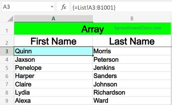
The formula: The formula below, is entered in the blue cell (A3), for this example
=List!A3:B1001
{=List!A3:B1001}
Source data from "List" tab:
Separate tab displaying referenced data/array:
Pop Quiz: Test your knowledge
Answer the questions below about array formulas, to refine your knowledge! Scroll to the very bottom to find the answers to the quiz.
Click the green "Print" button below to print this entire article.
Question #1
Which of the following formulas refers to a column of data?
- =A12:Z12
- =G1:G1000
- =B1
Question #2
Which of the following formulas refers to a row of data?
- =J3
- =U1:U1000
- =A9:Z9
Question #3
True or False: The following formula will not apply to an entire column, because the formula refers to a cell, instead of a range of cells:
=IF(D1=100,"Perfect","Not Perfect")
- True
- False
Question #4
Which of the following formulas refers to a range in another sheet?
- =A1:Z1000
- =Values!A3:B1000
Question #5
Which of the following formulas refer to a range with multiple columns? (Select all that apply)
- =Values!A:B
- =A:A
- =C:B
- =List!G:G
- =Y:Z
Question #6
Which of the following formulas will apply a multiplication formula to an entire column?
- =A3:AxB3:B
- =A3:A*B3:B
- =A3:A+B3:B
- =A3:A(B3:B)
Question #7
True or false: In some versions of Excel, to use an array formula, you need to hold Ctrl + Shift + Enter on the keyboard to enter the array formula.
- True
- False
Answers to the questions above:
Question 1: 2
Question 2: 3
Question 3: 1
Question 4: 2
Question 5: 1, 3, 5
Question 6: 2
Question 7: 1