

In Google Sheets, there is an easy way to format numbers in “Currency” format, without having to manually type the dollar sign when you enter numbers into the spreadsheet. Before knowing there is such an easy way to do this, many people either leave their numbers that represent money in plain number format, or they manually type dollar signs each time a number is entered.
But you can format the cells so that when new numbers are entered into the cell they automatically register as currency / money, and you can also convert existing numbers to currency format instantly. In this lesson I will show you how to format the cells in currency format, and I will also show you how to use a formula to format values as currency.
For example, if you want the number 1.25 to display as $1.25, simply change the format of the cell that contains the number, to “Currency”.
To format values as currency in Google Sheets, follow these steps:
- Select the cells that you want to convert to currency format
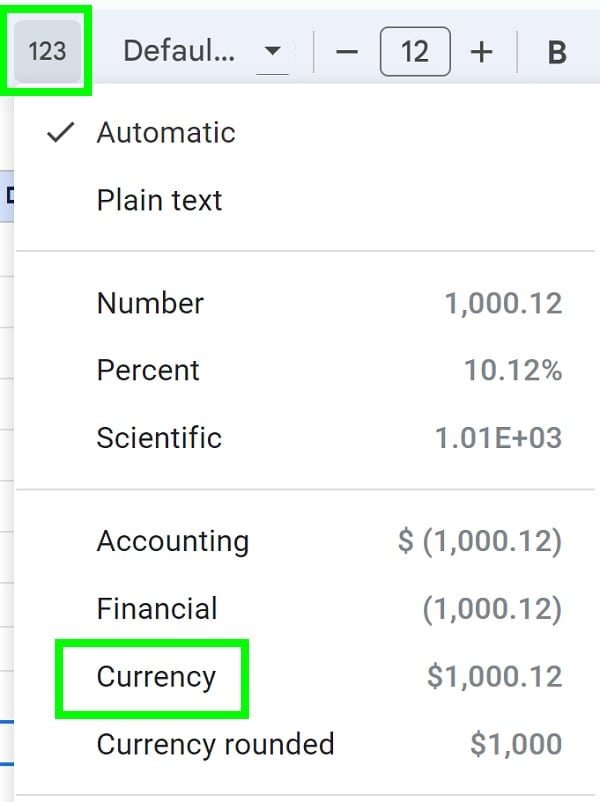
- On the top toolbar, click the “More formats” menu (The button has the numbers “123” on it)
- Click “Currency”
After following the steps, the values in the selected cells will display in the currency format with a dollar sign before the value, and numbers that you enter into those cells in the future will also display in currency format.
Now let’s go over examples of formatting values as currency, by using two different methods.
Using the “More formats” menu to format values as currency
In this example, we will use the menu option that allows you to change the format of the cells, so that the values in the cells appear in currency format, with a dollar sign that displays before the numbers.
When using currency format, the dollar sign is simply displayed in the cell and is not a part of the actual value / string that is entered into the cell. In other words the dollar sign is just for show, it does not get in the way of the calculations like other non-number characters would.
In this example we have numbers that are entered into columns A and B. The same numbers are listed in each column, so that you can see that difference before and after we convert to currency format. We are going to change the cells in column B to “Currency” format.
To do this, first select column B.
Then click the button on the top toolbar that says “123″ (When you hover over this button, the text “More formats” will pop up).
Choose “Currency”
As you can see in the image below, after following the steps to convert the cells to currency format, column B is formatted as currency, and displays a dollar sign before each of the values. These dollar signs were not entered manually, they automatically appeared when the cells were converted to currency format.
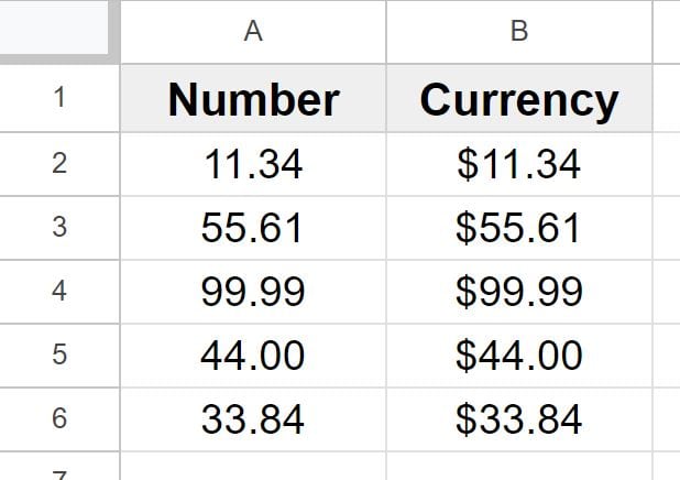
Cell A2 contains the number “11.34”, and cell B2 displays “$11.34”.
Using the TO_DOLLARS menu to format values as currency
If you want, you can use a formula to make your values appear in currency format in a Google spreadsheet. The formula that we used to do this is the TO_DOLLARS function.
To format values as currency by using a formula, follow the steps:
- Type =TO_DOLLARS( to begin the formula
- Type the number, or the address of the cell that contains the number that you want to convert to currency
- Press “Enter” on the keyboard. The formula will look like this: =TO_DOLLARS(1.25) or like this when using cell references =TO_DOLLARS(A2)
After following these steps, the formula will display the value that was specified as currency, with the dollar sign that displays before the value.
In this example, plane numbers are entered into column A, and we are going to convert the numbers to currency format by using a formula. To do this we will simply refer to the cells that contained numbers, with the TO_DOLLARS function.
=TO_DOLLARS(A2)
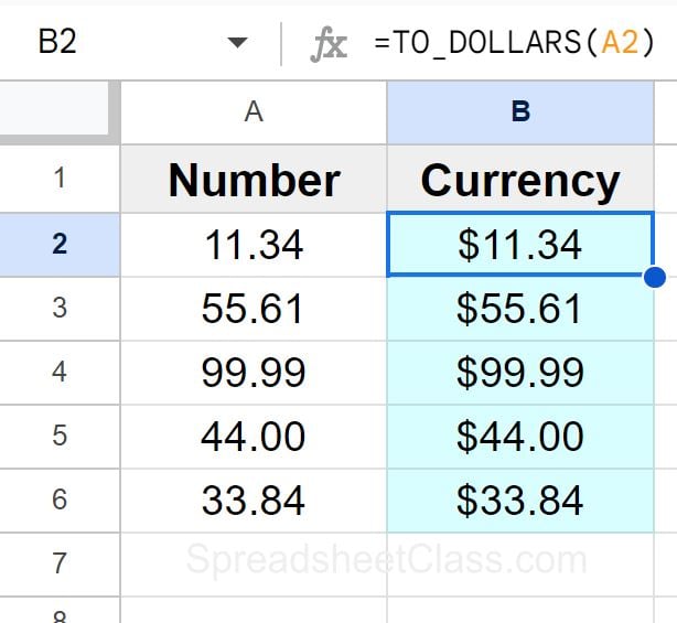
As you can see in the image above, cell A2 displays the number “11.34”, and the formula in cell B2 displays the value “$11.34”.
Increasing and decreasing decimal places from currency
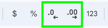
By default, when you convert to currency format, Google Sheets will automatically display two decimal places. You can increase or decrease the number of decimal places of your currency values by clicking “Increase decimal places”, or “Decrease decimal places”.
When dealing with currency values I often decrease the number of decimal places to show only the whole dollar amounts, since this looks cleaner in the spreadsheet and cleaner when the data is displayed on charts.
Below you can see what the decimal place buttons look like on the top toolbar.
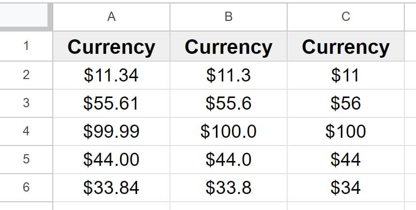
In the image below, you can see three different columns that contain the same numbers (in currency format), where column A has two decimal places, column B has one decimal place, and column C has 0 decimal places.
Now you know both ways to format the values in your Google spreadsheet as currency / money format!