How to convert currency in Google Sheets (Detailed examples)

Did you know that there is a Google Sheets formula that will allow you to convert from one currency to another? The GOOGLEFINANCE formula allows you to convert currencies, and stays up to date with changing conversion rates. For example, if you want to convert from U.S. Dollars to Euros, you can do this with the GOOGLEFINANCE function.

In this lesson I am going to show you how to convert from one currency to another in your Google spreadsheet, including how to retrieve the conversion rate as well as how to use the conversion rate to convert an amount of one currency to the corresponding amount of another currency.

Note that the GOOGLEFINANCE function can do other cool things such as pulling stock prices, but in this article we will focus on converting currency.

Converting currency with the GOOGLEFINANCE function

Now let's go over an example of converting from one currency to another currency. In this example we are going to use the GOOGLEFINANCE function to convert from U.S. Dollars (USD) to Euros (EUR).

When we specify the currency pair that we are converting between, we simply type the first currency code followed by the second currency code, with no spaces or characters between them, like this: USDEUR

To convert currencies in Google Sheets, use the GOOGLEFINANCE function like this =GOOGLEFINANCE("CURRENCY:Currency1Currency2") where "Currency1" is the 3-letter currency code of the currency you are converting from, and where "Currency2" is the three-letter currency code of the currency you are converting to. The final formula will look like this =GOOGLEFINANCE("CURRENCY:EURUSD")

The entire criteria for the function looks like this: "CURRENCY:USDEUR"

This tells Google Sheets to retrieve the conversion rate between two currencies (U.S. Dollars and Euros).

=GOOGLEFINANCE("CURRENCY:USDEUR")

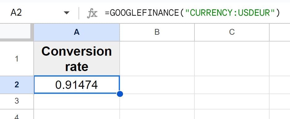
As you can see in the image above, the formula entered into cell A2 shows that the conversion rate for the USD / EUR currency pair was 0.91474 (at the time the image was captured).

A conversion rate of 0.91474 means that each unit of the first currency (USD) is worth 0.91474 of the second currency (EUR). So in this example every U.S. dollar is equivalent to 0.91474 Euros.

Later I will show you how to use this conversion rate to find the actual amounts when converting currencies, but first let's go over how to use cell references in these currency conversion formulas.

Check out this lesson if you want to learn how to format values as currency.

Using cell references to convert currency

If you want, you can use cell references when converting currencies with the GOOGLEFINANCE function. This will allow you to enter the three letter currency code into the cells, instead of having to type them directly into the formula. This makes it easy to change the codes for the conversions.

In this example, the first currency code (the currency that we are converting from) is entered into cell A2, and the second currency code (the currency that we are converting to) is entered into cell B2. We will refer to these cells to specify the currency pair that we are converting between in the GOOGLEFINANCE function.

To do this, we will use the ampersand (&) / "And" symbol, to combine the contents of two cells, since the symbols need to be placed "side by side" in a string.

So this portion of the formula "A2&B2" combines the contents of cell A2 and cell B2, which combines the two currency codes into a single string like we want (Example: USDEUR).

The entire formula criteria will look like this: "CURRENCY:"&A2&B2

This tells Google Sheets to combine the text string "CURRENCY:" with the currency codes that are entered into cells A2 and B2.

We will use the formula below to convert currencies by using cell references.

=GOOGLEFINANCE("CURRENCY:"&A2&B2)

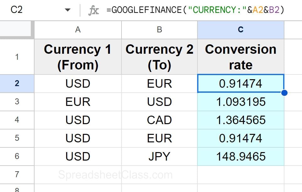
As you can see in the image above, cell C2 displays the conversion rate between the two specified currencies, and this was done by using cell references which means that the currency codes in cells A2 and B2 can be changed easily, to quickly change the currencies that the formula converts between.

You can also see that in the rows below, columns A and B have other currency codes, and the formula was copied down column C to calculate the conversion rate between a variety of currencies.

Finding the converted currency amount (Multiplying rate by the amount)

Now that you know how to find the conversion rate between two currencies, let's go over how to actually convert one amount of currency to another, given the conversion rate.

The conversion rate represents how many units of the second currency is equivalent to one unit of the first currency, and so we can use this conversion rate to convert amounts of currency by multiplying the conversion rate by the amount of the first currency. (Conversion rate x Amount of currency 1 = Amount of currency 2)

In this example, column A contains the codes for the currencies that we are converting from, and column B contains the amount / units of currency to be converted from. Column C contains the codes for the currencies that we are converting to.

First, we will use the GOOGLEFINANCE function to find the conversion rate between the first and second currency, and then we will multiply the conversion rate by the amount / units of the currency we are converting from so that we can calculate what the equivalent amount is for the currency we are converting to.

So row 2 shows that we are converting 100 U.S. dollars to Euros. Cell A2 contains the currency code "USD", cell B2 shows that we are converting $100, and cell C2 contains the currency code "EUR".

In cell E2, we will find the conversion rate with the formula below:

=GOOGLEFINANCE("CURRENCY:"&A2&C2)

In cell D2 we will find the number of Euros that are equivalent to the given amount of U.S. dollars by using the formula below, which multiplies the conversion rate by the amount of the first currency:

=B2*E2

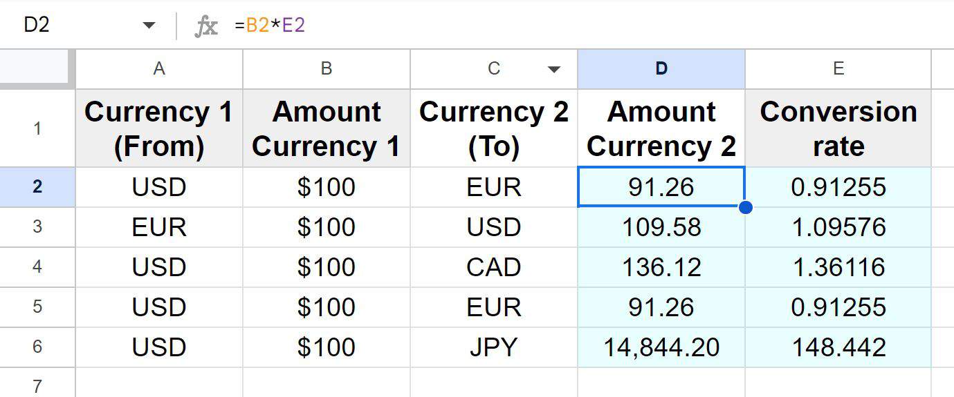
As you can see in the image above, cell E2 shows that the conversion rate between USD and EUR was 0.91255 (at the time the image was captured), and cell D2 shows that the conversion rate multiplied by the amount of currency 1 ($100) is 91.26, meaning that 100 U.S. dollars was equivalent to 91.26 Euros.

So the conversion rate shows you how many units of currency 2 are equivalent to one unit of currency 1, which means that you simply multiply by the units / amount of currency 1 by the conversion rate to find the units / amount of currency 2.

Converting back to the original currency

There are two ways that you can convert back to the original currency, or in other words there are two ways that you can switch the currencies you are converting from / to.

First, you can change the currency pair, to swap the currency codes, so that USDEUR becomes EURUSD, and vice versa. Or when using cell references, you can either change the cell references in the formula, or you can swap the currency codes that are in the cells while keeping the formula the same.

Second, you can divide by the conversion rate (instead of multiplying) if you don't want to change the order of the currency pair. For example, if the conversion rate for the currency pair USDEUR is 0.91255, and if you want to convert from Euros to U.S. dollars without changing the currency pair order, you can divide by the conversion rate. In this example, if you have 91.26 (decimal continues) Euros, and the conversion rate from USD to EUR was 0.91255, then you could divide 91.26 by 0.91255 to get the amount of USD that is equivalent to 91.26 EUR ($100 at the time this example was made).

So you can either switch the order of the currency pair, or divide instead of multiply by the conversion rate to convert in opposite order.

3-letter currency codes

3-letter codes that represent currencies are standard codes that are not unique to spreadsheets. Below are some of the more popular currencies and their associated 3-letter codes:

• AUD = Australian Dollar
• CAD = Canadian Dollar
• EUR = Euro
• JPY = Yen
• USD = US Dollar

Now you know how to not only find the conversion rate between two currencies, but you also know how to convert amounts of one currency to the corresponding amount of another currency in your Google spreadsheet.