

In Google Sheets there are several different ways to format dates. In this lesson I am going to show you the different options for date formatting that Google Sheets provides, and I’ll show you how to use custom date formats so that you can display your dates in the exact way that you want / in a way that makes sense for your data or presentation.
You can format dates to display the days, months and years in whatever order that you want, you can choose to display dates in text or numbers, you can choose to display the date of the week, or the time, and more.
Dates in a spreadsheet are simply numbers, and so changing the format of a date does not change the actual value, but simply displays the same value in a different format.
To change date format in Google Sheets, follow these steps:
- Select the cells containing the dates that you want to format
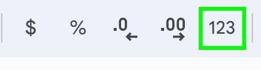
- Click “More formats” on the top menu which is a button that says “123” (Or you can click “Format” > “Number”)
- Choose the date format that you want. Google Sheets displays a preview of each format
After following the steps above, the date format in the selected cells will change according to your selection.
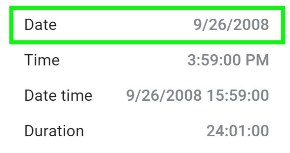
The image below displays what the “More formats” menu looks like.
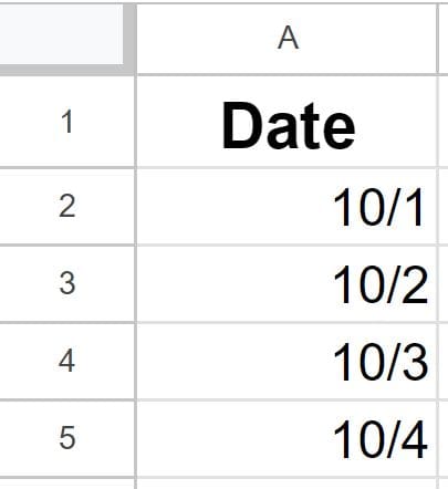
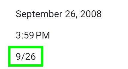
The default date format for Google Sheets contains the month and the day as shown below. Later I will show you how to return to the default format after changing the date format.
Default date format example: 10/1
Display date with year
First let’s go over how to change the date format to display the date with the year.
To display the date with the year in Google Sheets, follow these steps:
- Select the cells or columns containing the dates that you want to format
- Click “More formats” on the top menu (button that says “123”) Or you can click “Format” > “Number”.
- Choose the “Date” format that displays the date with the year
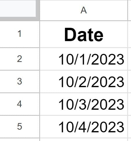
As you can see in the image below, after selecting the “Date” format that displays the date with the year, the dates now contain the year, and look like this: 10/1/2023
Display date without year (Default date format)
If you want you can select a date format that does not include the year, to make the dates smaller and more concise.
To display the date without the year Google Sheets, follow these steps:
- Select the cells or columns containing the dates that you want to format
- Click “More formats” on the top menu which is a button that says “123” (Or you can click “Format” > “Number”)
- Choose a date format that displays the date without the year

The default date format is an example of a date format that does not display the year, as shown in the image above.
Display date with month as text
If you want, you can display the month as text instead of a number in the date format. For example, you can display the month as “September” instead of “09”.
To display the date with the month as text in Google Sheets, follow these steps:
- Select the cells or columns containing the dates that you want to format
- Click “More formats” on the top menu (button that says “123”) Or you can click “Format” > “Number”.
- Choose the date format that displays the date with the month, where the month is shown as text
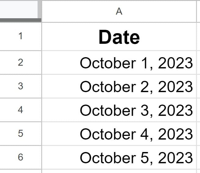
As you can see in the image below, after selecting the date format that displays the month as text, the dates now contain the month displayed in text, and look like this: October 1, 2023
Display date with time, by using date-time format
In some situations, you may need to include both the date and time in your dates, which is known as a date-time format. This is common for data that contains timestamps.
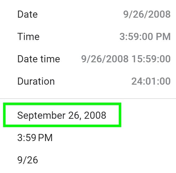
Date time format first displays the date, followed by the time, like this: 10/1/2023 2:24:00
The date time above represents October the 1st, in the year 2023, at 2:24 time with 0 seconds. (M/D/Y H:M:S)
To display the date with the time in Google Sheets (“Date time” format), follow these steps:
- Select the cells containing the dates that you want to format
- Click “More formats” on the top menu which is a button that says “123” (Or you can click “Format” > “Number”)
- Choose the “Date time” format that displays the date with the time
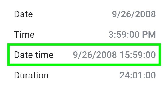
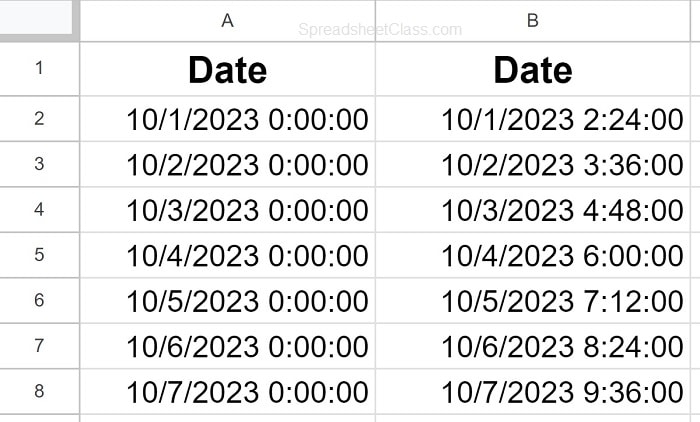
As you can see in the image below, after selecting the “Date time” format that displays the date with the time, the dates now contain the time, and look like this: 10/1/2023 2:24:00
Display date without time
If the dates in your spreadsheet display the time, and you do not want the time / only want the date to display, you can do this by changing the date format. The time value will still be available if you change the format back to date time, similar to when you display fewer decimal places in the cell, the decimal values are still stored in the background.
To display the date without the time in Google Sheets, follow these steps:
- Select the cells or columns containing the dates that you want to format
- Click “More formats” on the top menu (button that says “123”) Or you can click “Format” > “Number”.
- Choose a date format that displays the date without the time
The default date format is an example of a date format that does not display the time, as shown in the image above.
Change date format in Google Sheets to another locale
You can also adjust the date format to match the date conventions of different locales. This can be particularly useful when you’re dealing with international data or need to display dates in a specific regional format.
Each locale has its own date conventions, such as the order of day, month, and year.
To change the date format in Google Sheets to another locale, follow these steps:
- Click “File”
- Click “Settings”
- Navigate to the “General” tab
- Choose the desired country / locale from the “Locale” dropdown menu
- Click “Save settings”
After following the steps above, the date format in your Google Sheets document will be adjusted to match the conventions of the selected locale. This ensures that dates are displayed in a way that aligns with the regional standards of your choice.
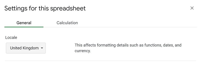
As you can see in the image above, “United Kingdom” has been selected, which will display dates in the format that corresponds with the United Kingdom.
Using custom date formats
While Google Sheets provides a variety of built-in date formats, you may encounter situations where you need a unique or specific date format that isn’t covered by the standard options. In such cases, you can create your own custom date format to precisely control how dates are displayed.
In the “Custom date and time” menu, you can choose from even more date formats, or you can create your own unique format.
To use custom date formats in Google Sheets, follow these steps:
- Select the cells containing the dates that you want to format
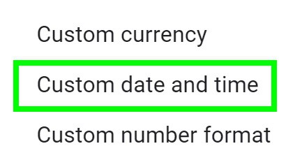
- Click “More formats” on the top menu
- Select “Custom date and time”
- Choose one of the existing date formats, or customize your own
- To customize a date format, choose from the items in the dropdown at the top, and separate each item with a space or a comma in the box that displays the custom date format. Select the items in the order that you want them to appear
- Modify the format as needed until it is as you want it to be. You can click anywhere in the box and delete items as if you were deleting text, and then you can add new items in any position that you want by placing your cursor where you want the item to be
- Click “Apply”
After following the steps above, the dates in the selected cells will be displayed according to your custom date format. This feature gives you precise control over the appearance of dates in your spreadsheet. If you need to edit the date format again you can do this easily by following the same steps above.
What I often do to create a custom date format, is select one of the existing formats that contains the elements / items that I want, and then I will delete any extra ones that I don’t want. Or sometimes I will simply click on the date formats to see the items appear in the box at the top to get a better understanding of how dates are formatted.
As you can see in the image below, a custom date format has been selected, which displays: Day of the week, month (as text), day , and the year.
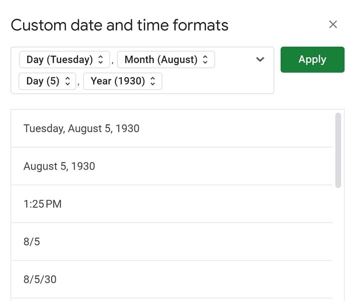
As you can see in the image below, after applying the custom date format, the dates now contain the chosen elements, and look like this: Tuesday, October 3, 2023

Display date with day of week
A very useful date format in Google Sheets displays the day of the week (Saturday, Sunday etc.).
To display the date with the day of the week in Google Sheets, follow these steps:
- Select the cells containing the dates that you want to format
- Click “More formats” on the top menu which is a button that says “123” (Or you can click “Format” > “Number”)
- Select “Custom date and time”
- Choose the date format that displays the day of the week
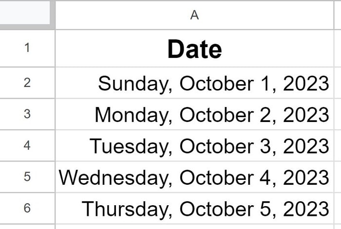
As you can see in the image below, after selecting the date format that displays the date with the day of week, the dates now contain the day of the week, and look like this: Sunday, October 1, 2023
Now you know how to format dates in Google Sheets, to display your dates in the exact way that you want!
How to remove date formatting
To remove date formatting, select the cells that you want to remove the date format from, click the “More formats” menu (Button says “123”), then choose “Automatic”, or another format that you want such as “Number”.
This will prevent Google Sheets from turning numbers into dates.