How to convert dates to text in Google Sheets

Are you looking for a way to convert dates into text in your Google spreadsheet? Whether you want to display dates in a specific format or combine them with additional text, this article will guide you through the process. We'll go over three methods: Using the TEXT function to convert a date to text, formatting cells as "Plain text", and using the CONCATENATE or "&" operator to merge dates and text into a single text string.

To convert dates to text in Google Sheets, follow these steps:

1. Select the cell or cells containing the date you want to convert
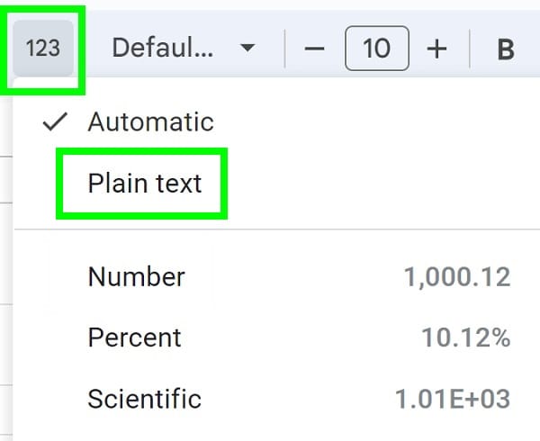
2. Click on the "More formats" menu in the top toolbar (The button says "123")
3. Click "Plain text"

After following the steps above, the dates in the selected cells will be converted into plain text format.

To convert dates to text with the formula, use the TEXT function like this: =TEXT(A1, "mm/dd/yyyy")

Now let's go over some detailed examples of how to convert dates to text in Google Sheets in a variety of ways.

Using the TEXT Function to convert a date to text

With the TEXT function, you can automatically convert dates to text, in any format that you want.

To use the TEXT function, first you specify the cell that contains the value that you want to convert to text, and then you specify the format. There are a variety of ways to specify the format when converting a date to text, which I will show you below.

To use the TEXT function to convert a date to text, follow these steps:

1. Select the cell where you want to display the date as text
2. Type =TEXT( to begin your formula
3. Type the cell reference or date value that you want to convert to text. For example, if the date is in cell A1, your formula would look like this: =TEXT(A1
4. Type a comma, and add a text string within double quotation marks ("). This string should contain placeholders for the parts of the date you want to display. You can use various codes to represent the date elements, such as "dd" for the day, "mm" for the month, and "yyyy" for the year
5. Press "Enter" on the keyboard. Your formula should look like this: =TEXT(A1, "mm/dd/yyyy")

After following the steps above, the selected date in the cell will be converted into the specified text format.

Before we move on, let's go over how to format the dates exactly how you want with the TEXT function. Below are the different ways that you can specify months, days, and years. You can mix and match them in any order that you want, and you can choose if you want spaces or commas or forward slashes (/) between each of them.

The Google Sheets TEXT function description:

Syntax:
TEXT(number, format)

Formula summary: “Converts a number into text according to a specified format.”

Let's say that you have a spreadsheet with a column of dates, and you want to convert these dates into a text format of your choice.

In this example, cell A2 contains the date "10/29/2023." What we are going to do is convert this date into text format, so it appears as "October 29, 2023." To do this, we will use the TEXT function as explained in the steps above.

In cell B2, enter the formula =TEXT(A2, "MMMM DD, YYYY"). After pressing Enter, you will see that cell B2 now displays the date in the desired text format: "October 29, 2023" as shown in the image below.

=TEXT(A2, "MMMM DD, YYYY")

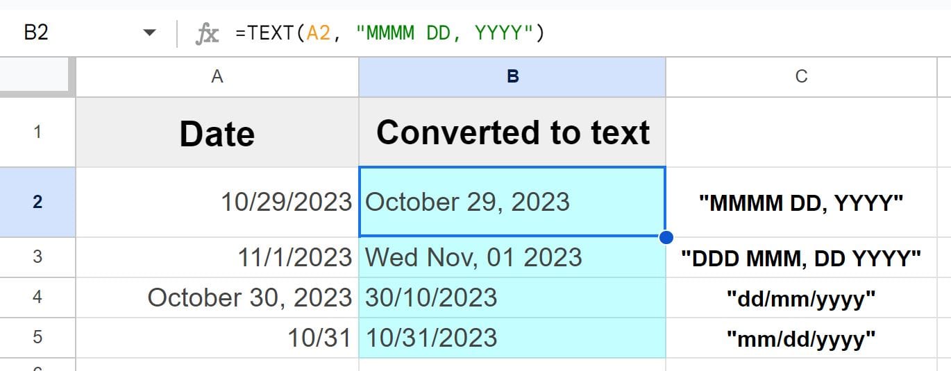
In the image above, you can see a variety of examples where the dates are formatted in different ways after being converted to text. You can choose whether you want to display the days and months as numbers or as text, you can choose to put the day, month, and year in whatever order that you want, and you can choose whatever characters that you want to separate the days, months, and years.

Notice that it does not matter whether you capitalize the letters or not when specifying the date format for days, months, and years. Also notice that the original dates in column A are in a variety of formats, but this will not affect the result of the TEXT function because no matter what format the date was originally in, with the TEXT function you set exactly how you want the format to be in the cell that has the formula.

Example date formats for the TEXT function:

• "MMMM DD, YYYY"
• "DDD MMM, DD YYYY"
• "dd/mm/yyyy"
• "mm/dd/yyyy"

Format the cells as "Plain text" to convert a date to text in Google Sheets

A very simple way that you can convert dates to text in a spreadsheet, is by simply changing the format of the cells to "Plain text" format.

When you do this, Google Sheets will convert the date displayed in the cell to text, displayed in the same visual format that the original date was in.

When using this method, if you want the date to appear in a specific format after the cells are converted to plain text format… first convert the cells to the desired date format, and then convert the cells to plain text.

To format the cells as "Plain text" to convert a date to text, select the cell or cells containing the date(s) that you want to convert to text, click on the "More formats" menu in the top toolbar (The button says "123"), then click "Plain text".

After following the steps above, the selected date(s) will now be considered as text by Google Sheets, although they will appear the same in the cell.

Let's say that you have a spreadsheet with a column of dates, and you want to convert these dates into a plain text format without using a formula. In this example, we have a column where cells A2:A6 contain the date "10/29/2023" in a variety of different formats. What we are going to do is format the cells as "Plain text" so that they displays the dates as a simple text string.

To do this, we will use the steps outlined above.

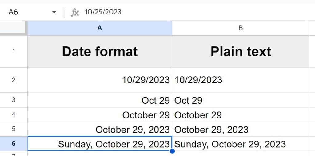
In the image above, there are multiple important things to notice. First of all, you can see that column A is aligned to the right, and column B is aligned to the left, this was not done by specifically choosing the alignment, this happened because by default dates are aligned to the right of the cell just like numbers, but when they are converted to text they will be aligned to the left, as shown in the image which shows a variety of examples of dates in different formats.

Also, notice that Cell A6 displays a different format in the cell itself, as it does in the formula bar. The cell shows "Sunday, October 29, 2023" where the formula bar shows "10/29/2023". This is because the dates in column A are in date format, and Google Sheets is displaying the default format in the formula bar.

But when you click on Cell B6, the value displayed in the cell will be the same value that is displayed in the formula bar. This is because the dates in column B were converted to text, and Google Sheets is interpreting the string as text like we want.

Using CONCATENATE or "&" operator to combine dates and text into a string in Google Sheets

If you want you can combine dates with text to make a customized string of text that includes a date.

To do this we can use the CONCATENATE function, or the "&" operator (called an ampersand). Below I will show you both methods.

To use CONCATENATE to combine dates and text into a string, follow these steps:

1. Type =CONCATENATE(
2. Enclose the text you want to insert in quotation marks. For example: "Date: "
3. Reference the cell that contains the date you want to combine with the text
4. Press "Enter"

After following the steps above, the selected cell will display the date combined with the specified text.

Let's say that you have a spreadsheet with a column of dates, and you want to add a label "Event Date: " before each date.

In this example, we have a column where cell A2 contains the date "10/29/2023."

What we are going to do is use the CONCATENATE function to combine the text "Event Date: " with the date in cell A2. To do this, we will use the steps outlined above.

=CONCATENATE("Event Date: ",A2)

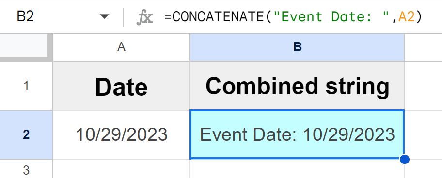
As you can see in the image above, the date and cell A2 has now been combined with the specified texturing, so that cell B2 now displays "Event date: 10/29/2023".

It's important to note that when using this method, the cell that contains the date you are combining with the text string must be in plain text format, or Google Sheets will read the date as a number and will combine the specified text string with a number instead of displaying the date like you want, like this "Event date: 45228".

So you can either convert the cell that contains the date to plain text, or you can use the formula below to convert the date to text with the formula. This combines the CONCATENATE function with the TEXT function.

=CONCATENATE("Event Date: ",text(A2,"mm/dd/yyyy"))

Now let's go over how to do the same thing by using the "&" operator instead of the CONCATENATE function.

To use the "&" operator to combine dates and text into a string, follow these steps:

1. Type an equals sign (=)
2. Enclose the text you want to insert in quotation marks. For example: "Date: "
3. Type an ampersand (&)
4. Reference the cell that contains the date you want to combine with the text
5. Press "Enter"

="Event Date: "&A2

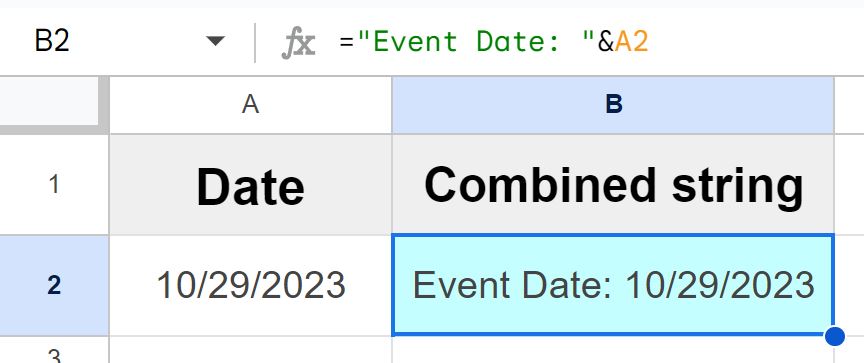
As you can see in the image above, this formula does the same thing as the CONCATENATE formula does.

Make sure that the cell that contains the date you were combining with the text is in plain text format, or you can use the formula below to convert the date to text. This will make sure that the date displays in the desired format when you combine it with the text, instead of displaying as a number.

="Event Date: "&text(A2,"mm/dd/yyyy")

Converting multiple dates / entire columns of dates to text in Google Sheets

Now that you've learned the methods for converting dates to text in Google Sheets, you can learn how to convert entire columns / ranges of dates to text. In this section, we'll discuss how to copy formulas down a column, and how to format an entire column as "Plain text."

Copying the TEXT formula down a column

Suppose you want to use the TEXT function to convert a column with dates to text. You can do this by copying the formula at the top of the column into the cells below.

To copy the formula down the column, follow these steps:

1. Click on the cell that contains the TEXT formula that you want to copy
2. Hover your cursor over the small square in the bottom right corner of the selected cell, and your cursor will turn into a cross (this is called the "fill handle")
3. Click and drag the fill handle down to copy the formula into all the cells / rows that you want the formula copied into

After following these steps, your TEXT formula will be applied to each cell in the column, and Google Sheets will automatically adjust the cell references for you.

If you want to apply the formula to the entire column by using a single formula, check out the article on using the ARRAYFORMULA function.

Formatting an entire column as "Plain text"

If you want, you can use the method that changes the format of the cells, to convert an entire column / range of dates to text.

To convert an entire column into text by formatting cells, follow these steps:

1. Click on the lettered header of the column containing your dates
2. Click the "More formats" menu in the top toolbar (The button says "123")
3. Click "Plain text"

These steps will format the entire column as plain text, converting all the dates within that column to text format.

Checking if a date is in text format

If you want to make sure that your date is in text format, or just to check whether it is or isn't, you can use a couple of methods to do this.

Use the ISTEXT function to check if the date is text

First you can use the ISTEXT function to check whether or not a specified value is text. Simply refer to the cell that contains the value that you want to check, and the ISTEXT function will display TRUE if the value is text, or FALSE if the value is not text, as shown in the image below.

=ISTEXT(B2)

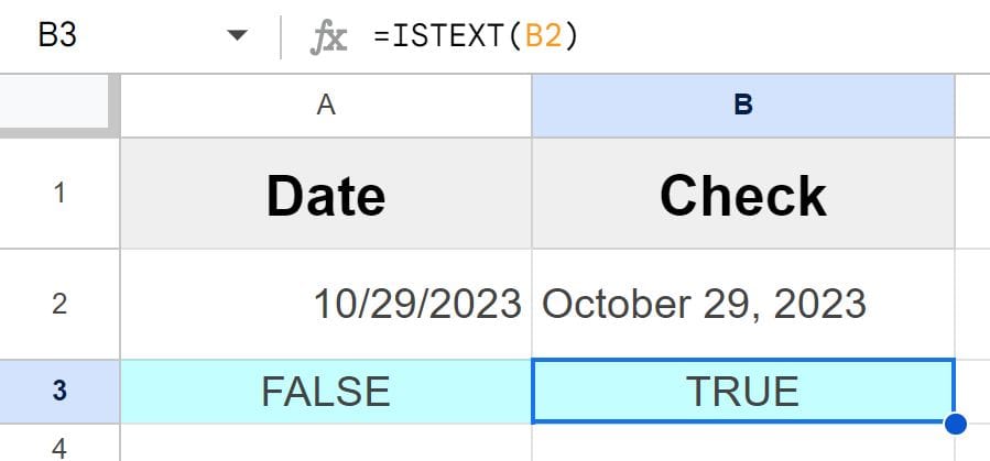
As you can see in the image above, the formula in cell B3 is checking to see if the date in cell B2 is in text format. Cell B3 displays the word TRUE which tells us that the date is in text format.

The ISTEXT formula in cell A3 checks the date in cell A2, and shows the word FALSE which tells us that the date is not in text format.

Check to see if a cell matches another cell

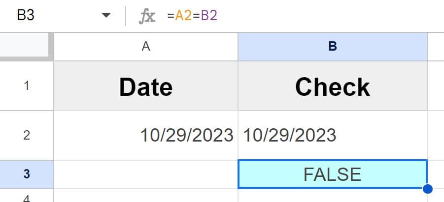
Another way that you can identify dates that are in text format, is to compare a cell that contains a date, to another cell that contains a date. This is something that I do when I am troubleshooting and making sure that my dates are in the same format. If the cells are equal to each other then the dates in those cells are in the same format.

To do this we use a formula like the one below, which simply asks Google Sheets if the value in one cell matches the value in another cell.

=A2=B2

Now you know all of the different ways to convert dates to text in Google Sheets, whether you want to use a formula or format the cells.

Click here to get your Google Sheets cheat sheet

Or click here to take the dashboards course