

In Google Sheets, sometimes you will find the need to calculate the number of days between two different dates, or to subtract days from a date to find what the date would be x many days ago. Since dates are simply numbers displayed in a special way in a spreadsheet, calculating the difference between dates is very easy. In this lesson I am going to show you how to find the number of days that there were between two dates, and I’ll also show you some really handy ways to calculate days elapsed / average days elapsed when dealing with multiple dates in your spreadsheet.
In a spreadsheet, a date is simply a number, and each time that a date increments by one day, in the background it is simply a number that is incrementing by one. So each day / each 24 hours is equivalent to the number one.
1 Day / 24 Hours = 1
So when you subtract today’s date from tomorrow’s date, the answer will be “1”, because there is 1 day between today and tomorrow.
Tomorrow’s date – Today’s date = 1
To calculate days between dates in Google Sheets, follow these steps:
- Type an equals sign (=)
- Type the address of the cell that contains the more recent date
- Type of minus sign (-)
- Type the address of the cell that contains the older date
- Press “Enter” on the keyboard. The final formula will look like this, where cell A2 is the more recent date, and cell A1 is the older date: =A2-A1
To subtract days from a date in Google Sheets, follow these steps:
- Type an equals sign (=)
- Type the address of the cell that contains the date
- Type of minus sign (-)
- Type the number that you want to subtract, or the address of the cell that contains the number that you want to subtract
- Press “Enter” on the keyboard. The final formula will look like this: =A1-5 (Or like this, where cell A2 contains the number to be subtracted: =A1-A2)
After following these steps, the cell with the formula will display the number of days between the specified dates.
This article focuses on finding the numbers of days between dates, and goes over a couple examples of subtracting days from dates, but you can also learn to add and subtract days to/from dates in Google Sheets in a variety of ways.
Click here to learn how to calculate the duration between two times.
Now let’s go over a variety of examples on calculating days between dates.
Calculate days between dates from cell to cell
Let’s start with the basic example of calculating the number of days between two dates.
As you can see in the image below, the date 11/1/2023 is entered into cell A2, and the date 11/3/2023 is entered into cell B2. Since the dates are so close together we can simply look at the dates and see that there are two days between these two dates. But we are going to set up a formula that automatically calculates this.
In cell C2, we enter the formula =B2-A2, which subtracts cell A2 from cell B2 (or in other words it subtracts the date that is in cell A2 from the date that is in cell B2). Remember that when calculating the days between dates / the difference between dates, the newer date is the date that you are subtracting from, and the older date is the date that you are subtracting.
=B2-A2
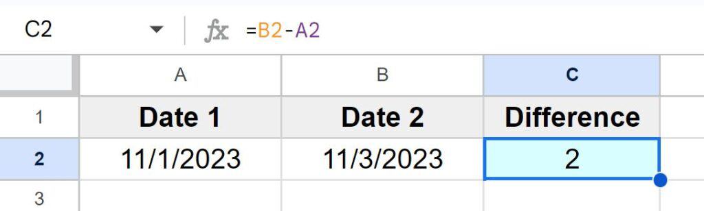
As you can see in the image above, cell C2 shows the number “2”, indicating that there are 2 days between the date 11/1/2023 and the date 11/3/2023.
Below I will show you a variety of ways to calculate days between dates when you have multiple dates in your spreadsheet.
Calculate days between multiple dates and average days between dates
Now let’s go over an example where we will calculate the days between dates given two columns of dates. Then we will find the average number of days between the dates in the two columns.
Column A contains the initial dates, and column B contains the new / final dates. We are going to use column C to subtract the dates in column A from the dates and column B, which will give us the number of days between the dates in each row.
Cell C3 contains the formula =B3-A3, which subtracts the date in cell A3 (3/1/2023) from the date in cell B3 (11/3/2023), and displays that there were 247 days between the two dates. Then we copy this formula down the column, and Google Sheets automatically adjusts the cell references to calculate the difference between the dates in each row, giving us the number of days between each date and each row.
The formula below is initially entered into cell C3, and then is copied down the column:
=B3-A3
The formula below is entered into cell C1:
=AVERAGE(C3:C)
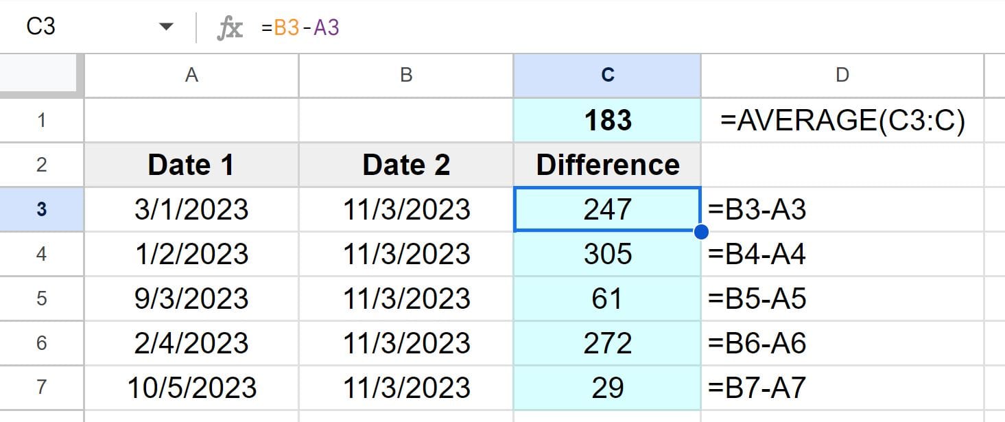
As you can see in the image above, the number of days between the dates in columns A and B are displayed in each row in column C. Then at the very top of column C, the AVERAGE function is used to calculate the average number of days calculated between the dates this is useful for situations such as when you want to calculate the average days that it takes to complete a project.
Days elapsed / days between dates from row to row
In this example, instead of calculating the number of days between two different dates in two different columns, we are going to calculate the number of days that have elapsed from row to row given a single column of dates.
To do this we will use a subtraction formula, and we will subtract the older date (previous row) from the newer date (current row)
To calculate days elapsed from row to row (cell to cell), subtract the date in the preceding cell (initial date) from the date in the succeeding cell (final date). When you copy the formula down the column, Google Sheets will automatically adjust the cell references to refer to the appropriate rows in each new formula / row.
The formula in each row will display the days between the date in the previous row and the date in the current row.
In this example, we have a list of dates in column A. What we are going to do is calculate the number of days between one row and the next. To do this, we use the following formula: =A3-A2. This formula starts in cell B3 and is copied down the column.
=A3-A2
The formula begins in cell B3 and not cell B2, because row 2 is where the first data point is, and there is not a previous data point that we can compare for calculating days elapsed.
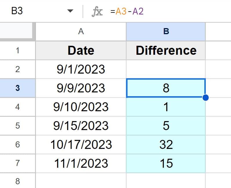
As you can see in the image above, cell B3 displays that there were 8 days between cell A2 (9/1/2023) and cell A3 (9/9/2023). The formula was copied down the column, and Google Sheets automatically adjusts the cell references, as shown below.
Cell B4 will have the formula: =A4-A3
Cell B5 will have the formula: =A5-A4
Cell B6 will have the formula: =A6-A5
If you want, you can find the average number of days between the dates with the AVERAGE function, like in the previous example.
Days elapsed from row to row (with a fixed starting point)
This example is going to be very similar to the last example, except in this case we are going to calculate the days elapsed from row to row by using a fixed starting point as the initial date. So we will calculate the days between the fixed starting date, and the date in each row.
In cell B3 we will calculate the days elapsed from the date in cell A2 to the date in cell A3.
In cell B4 we will calculate the days elapsed from the date in cell A2 to the date in cell A4.
In cell B5 we will calculate the days elapsed from the date in cell A2 to the date in cell A5.
In cell B6 we will calculate the days elapsed from the date in cell A2 to the date in cell A6.
The reference to cell A2 stays the same when the formula is copied into the cells below (because it is our fixed starting date / cell), but the other cell references increment by one row each time the formula is copied into a new row, so that each date in each row can be compared to the fixed to starting date.
To make it so that the cell reference to the initial dates / fixed starting date does not change when the formula is copied into cells below, we will put a dollar sign before the row reference, like this: A$2. This dollar sign will prevent the reference to the starting date from changing when the formula is copied.
=A3-A$2
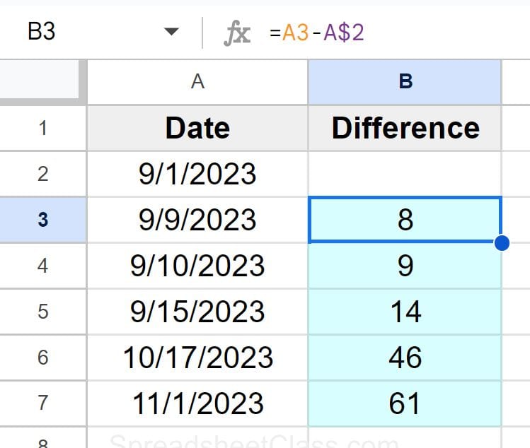
In the example image above, you can see that the date 9/1/2023 is entered into cell A2. There are other dates entered in column A, below cell A2. We want to find how many days elapsed between each of these dates and initial fixed starting date in cell A2.
By using the following formula (starting in cell B3) we calculate the days between cell A2 and cell A3: =A3-A$2
When we copy the formula (in cell B3) into cell B4, the formula will adjust so that the initial value / reference to cell A2 remains the same, while the row reference to cell A3 will increment by 1 row, as desired.
Cell B4 will have the formula: =A4-A$2
Cell B5 will have the formula: =A5-A$2
Cell B6 will have the formula: =A6-A$2
The formula calculates the days between the fixed starting point, and each date in each row below the fixed starting date.
Subtracting days from dates
Just like you can subtract one date from another to get a number of days between the dates… you can subtract a number from a date to get the date x many days before the original date.
Below I will go over two examples of how to subtract days from dates, but check out this Pro lesson that will teach you a variety of ways to both add and subtract days / months / years from dates in Google Sheets.
Earlier I mentioned how tomorrow’s date minus today’s date will give an answer of “1”. Much the same, if you subtract 1 from tomorrow’s date, this will give you today’s date. In other words, when you subtract a number from a date,the formula will give you the date that occurred that many days ago.
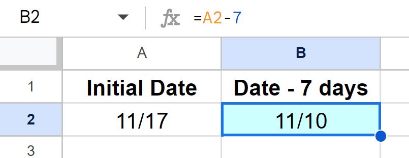
Subtract days from a date by using numbers
You can subtract days from a date by entering the number of days to subtract directly into the formula, as shown below. The initial date is entered into cell A2 (11/17) and cell B2 contains the formula =A2-7, which will subtract 7 days from the date that is in cell A2, and give the date that it was that many days ago (11/10).
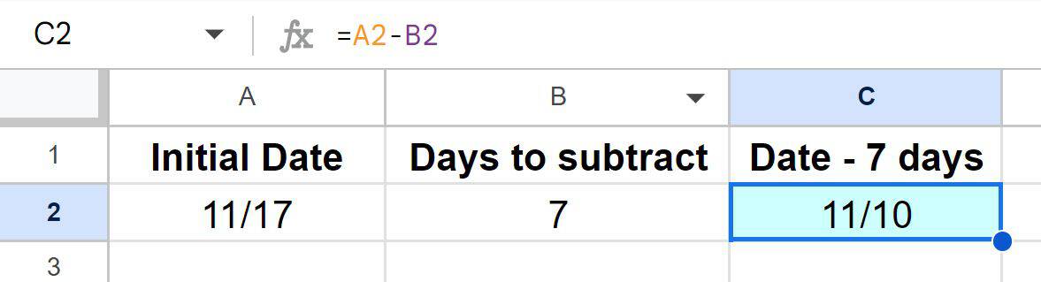
Subtract days from a date by using cell references
If you want, you can subtract days from a date by entering the number of days to subtract into a cell, and then referring to that cell in the subtraction formula, as shown below. The initial date is entered into cell A2 (11/17), cell B2 contains the number of days to subtract, and cell C2 contains the formula =A2-B2, which will subtract 7 days from the date that is in cell A2, and give the date that it was that many days before (11/10).
Now you know a variety of ways to calculate the number of days between dates in Google Sheets!