

Are you looking for a way to remove gridlines in Google Sheets? In this article I am going to show you how to remove gridlines, how to add them back again when they are missing, and I’ll also show you how to customize gridline color.
Personally I like to remove gridlines when I am building dashboards and want a clean background for my charts.
Gridlines are enabled by default in Google Sheets, but you can easily remove them to create a clean layout, such as when you want a tab to hold your charts, where the background is not too busy with lines everywhere.
To remove gridlines in Google Sheets, follow these steps:
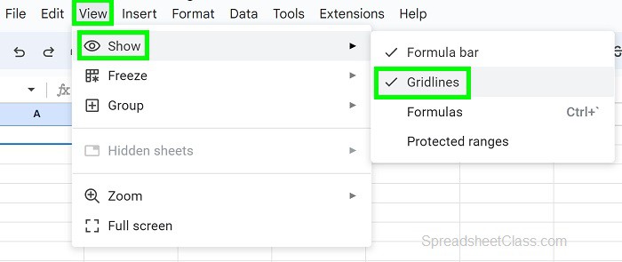
- Click “View” on the top toolbar
- Click “Show”
- Click “Gridlines”
After following the steps above, the gridlines will be removed from your sheet.
Removing gridlines is particularly useful when you add charts to your sheet and want the background to be clean, as demonstrated in the example below.
Removing gridlines from the entire sheet
Now let’s go over an example of removing gridlines in a Google spreadsheet. Let’s say that we want to remove the gridlines on an entire tab, so that the sheet is pure white.
- Click on the “View” menu located at the top of the spreadsheet
- Click (or hover over) the “Show” menu option
- Click “Gridlines.” By default, this option is checked, indicating that gridlines are visible
You’ll notice that the gridlines disappear, leaving you with a clean and grid-free view of your data.
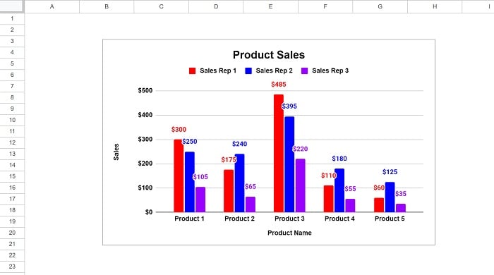
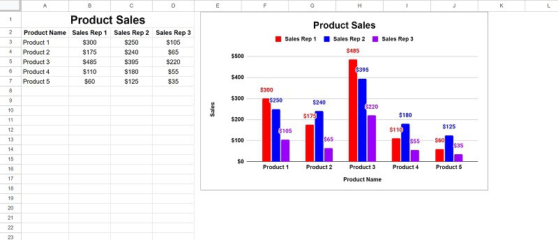
In this example we have a column chart on a tab, and we want to remove the gridlines from the tab so that the chart has a clean background.
As you can see in the image below, after removing the gridlines, the cells no longer have any borders and are pure white. This makes it very easy to view the chart without the gridlines in the background.
Add gridlines if they are missing
You can follow the same process if you want to enable gridlines again.
To add gridlines in Google Sheets, click “View”, then click “Show”, then click “Gridlines”.
A checkmark will display next to the word “Gridlines” when the feature is enabled.
Change gridline color
You can also customize the appearance of gridlines with unique colors or line thickness by using borders. In this example we are going to turn the gridlines / borders red, but you can choose any color that you want.
To change gridlines color in Google Sheets, follow these steps:
- Select the range to apply the color change to (or select the entire sheet by pressing Ctrl + A)
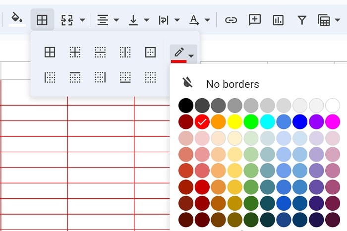
- Click the “Borders” dropdown (The button looks like a grid)
- Click “Border color”
- Select the desired gridline color
- Click “All borders” to apply the color change to the selected range / sheet
The gridlines of the selected cells will now be the color that you chose, as shown in the image below.
Note that the default gridlines are the color “Dark gray 4”, so if you turn your cells this same color the gridlines will not be visible.
Or you can simply match the border color with any fill color and the gridlines will not be visible.
Make gridlines darker
If you want to make the gridlines darker, you can make the color slightly darker by choosing black instead of dark gray, or you can change the border style to a thicker border. Making the border thicker actually makes a bigger difference because the default border style has such thin lines.
To make gridlines darker in Google Sheets, follow these steps:
- Select the cells to apply the color change to (or select the entire sheet by pressing Ctrl + A)
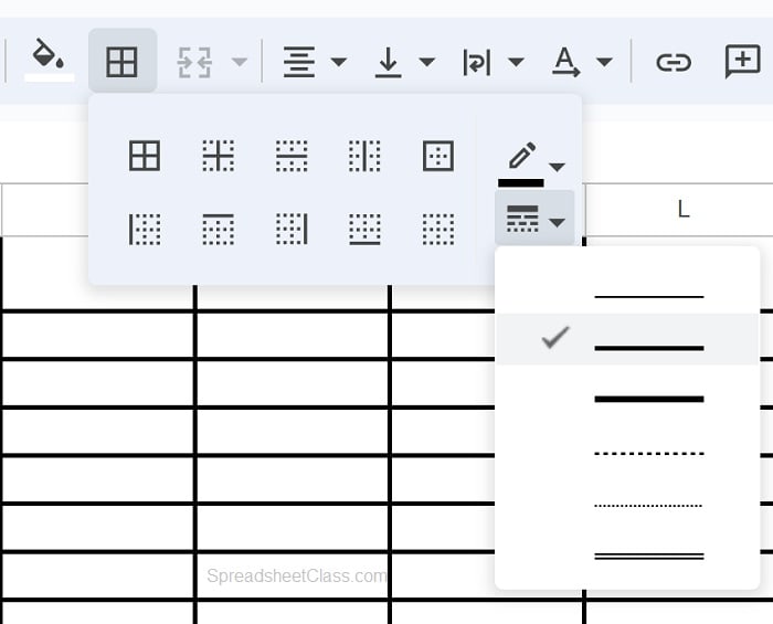
- Click the “Borders” button (Looks like a grid)
- Click “Border style”
- Select the desired border thickness
- Click “All borders” to apply the change to the selected range / sheet
- The gridlines of the selected cells will now be thicker and darker, as shown in the image below.
After following these steps your borders / gridlines will be thicker and will appear darker / will stand out more.
As you can see in the image above, the borders now appear darker since the thickness of the lines was increased.
How to insert / remove gridlines from specific cells
If there are certain parts of your sheet where you want to apply gridlines to, where you want the other parts of the sheet to have no gridlines, this can be done in two different ways.
Method 1: Remove the default gridlines from the entire sheet as explained in the first example (Click “View” > “Show” > “Gridlines”), and then add dark borders to the cells where you want gridlines.
Method 2: Keep the default gridlines and use white borders to remove the gridlines / borders from the desired parts of the sheet.
Now you know how to remove gridlines, how to add them back again, and how to customize gridlines too!