

If you are having issues with the SUM function in Google Sheets, whether it's not working or not showing the correct result, this article will show you how to fix the error.
There are several different ways that an error can occur with the SUM function, from setting up the formula incorrectly to formatting the data incorrectly.
Although there are a variety of detailed solutions below, the two most common errors that I have experienced with the SUM function are when data is in a format such as "Plain text" (instead of numbers), and when the references in my formula are slightly wrong. Make sure that the data that you are summing is formatted as numbers, and make sure that the references to rows and columns in your formula are correct.
Syntax errors
First check for any missing or extra parentheses, commas, or other characters in your SUM function. If extra unexpected characters are entered into a formula, this will cause an error.
Your SUM function should look like this =SUM(A1:A) or like this =SUM(A1:A100)
Make sure the cells are formatted as numbers and not text
Incorrect cell formatting will cause the SUM function to calculate incorrectly. When the values are formatted as text, the SUM function will not be able to sum those values. This can either cause the SUM function to display the wrong result, or it can prevent it from working at all.
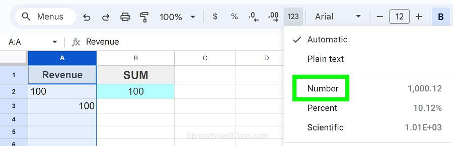
To make sure that your SUM function works properly, make sure that the data that you are summing is formatted as numbers. To do this, select the range of cells that you want to format as numbers, then on the top toolbar click "More formats" which is the button that says "123". Then click "Number". This will ensure that your data is interpreted as numbers so that the SUM function works properly.
With the default "Automatic" format, Google Sheets will automatically detect that the data is numbers, but sometimes the cells in a spreadsheet get formatted as text, and so you can change the format to "Number".
There are certain cases where the automatic format doesn't work as expected, such as when you are using a formula that refers to another range of cells, and the original range is formatted as text. In this case the automatic format will display the format of the original location, instead of automatically detecting the correct format. This is why it is good practice to specifically format cells as "Number" in the cells should be treated as numbers.
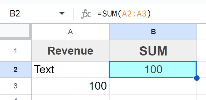
In the image below, you can see how the SUM function reacts when there is text in the column mixed in with numbers. The formula is summing the numbers in the column, and ignoring text. So if you have text or extra characters that were accidentally entered in a column that has numbers, the function will not display an error and will ignore the entry that has text, yielding a wrong result.
=SUM(A2:A3)
(Formula is correct in this example, but the data formatting is wrong)
Even when you enter numbers into a cell, if the cell is formatted as text, the SUM function will not recognize it as a number and will not calculate properly.
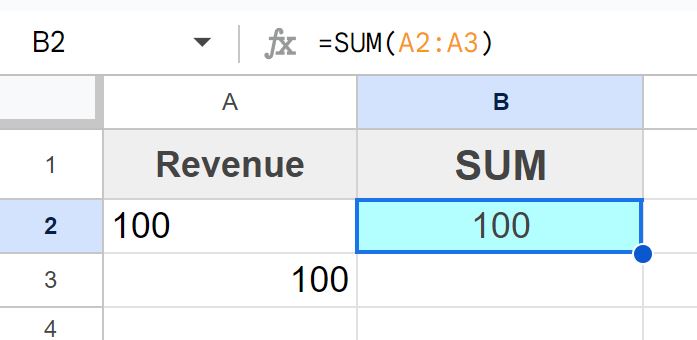
In the image below you can see that the number 100 is entered into cell A2, and the number 100 is entered into cell A3. The SUM function is summing cell A2 and A3, but it is giving us an answer of 100 when the answer should be 200. This is because cell A2 is formatted as "Plain text".
If a number that you entered is formatted as plain text, and you have not chosen an alignment for the cell, by default the value will align to the left side of the cell if it is formatted as text. The value will align to the right side of the cell if it is formatted as a number. So you can see that the number in cell A2 is aligned on the left because it was mistakenly formatted as text.
But if you specifically select an alignment for the cells, such as center aligning the values, if they are accidentally formatted as text the alignment will not change. So make sure that the cells / columns you are summing are formatted as numbers.
As you can see in the image below, column A is selected, and the "More formats" menu is open. Select "Number" from this menu.
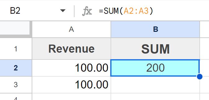
As you can see in the image below, after formatting column A as numbers, the SUM function is correctly summing column A, giving a result of 200 as expected.
Check the references
One of the most common ways that the SUM function will not work correctly, is when the wrong cell references are entered. Make sure that the SUM function is referring to the correct column, row, or range of cells. It may sound obvious but it's an easy mistake to make when you are rushing with a project.
When the beginning row is wrong
Notice in the image below that the data is in rows 2 through 6, but the SUM function starts summing on row 5. This is the incorrect row to begin on, so the total is not displaying the correct answer. To fix this, simply change the reference so that it begins on the correct row.
Incorrect formula:
=SUM(A5:A)
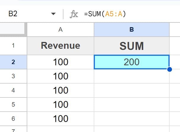
Corrected formula:
=SUM(A2:A)
When the ending row is wrong
The same error can occur when the wrong ending row is specified. This often happens when you refer to all of the rows in the sheet, but more rows are added if the SUM function is not adjusted accordingly.
As you can see in the image below, the data is in rows 2 through 6, but the SUM function is only summing rows 2 through 4. To fix this, simply change the reference so that it is referring to rows 2 through 6, or starting at row 2 through the entire column.
In Google Sheets you do not need to specify an ending row, and you can simply use a reference like this to specify an entire column / the remainder of a column: A2:A
I like to use this method so that the SUM function at the top of the sheet will calculate the entire column no matter how much data is added below.
Incorrect formula:
=SUM(A2:A4)
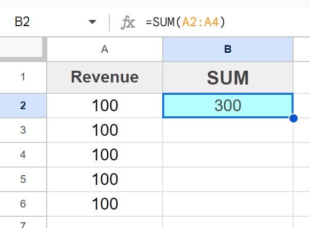
Corrected formula:
=SUM(A2:A)
When you refer to the wrong column
Sometimes the error that you experience with a SUM function may be as simple as referring to the wrong column. Make sure that your SUM function is referring to the correct column that you want to sum.
When you accidentally refer to multiple columns
Sometimes you may accidentally refer to multiple columns with the SUM function when typing your references. If the SUM function refers to multiple columns, it will sum all of the cells in both columns, which will give an unexpected answer if that's not what you meant to do and both columns contain numbers.
If you want to SUM column A, make sure that your formula does not look like the formula directly below which sums both columns A and B.
=SUM(A2:B)
The formula below correctly sums a single column.
=SUM(A2:A)
Fixing a circular dependency error with the SUM function
Circular dependency errors can occur when using the SUM function in the spreadsheet, especially when your SUM function is at the bottom of your data instead of the top.
A circular dependency means that the formula has a reference that refers to the cell that the formula is in. In other words the formula is referring to itself. This causes an error called a "Circular dependency".
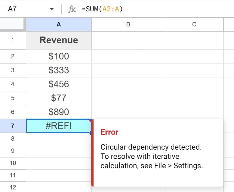
When this occurs Google Sheets will display #REF! in the cell with an error / the cell that contains your SUM function.
As you can see in the image below, the SUM function and cell A7, is attempting to sum the range A2:A. Cell A7 is inside of the range A2:A, and so this causes a circular dependency error since the formula is inside of the range that the formula is referring to. This basically means that the output of the input of the function would be dependent on the output, which is not possible.
Formula causing the error:
=SUM(A2:A)
The circular dependency error can be fixed by either moving your formula to a different location in the spreadsheet, or by changing the references in the formula. In either case, make sure that the formula is not referring to itself or in other words make sure that the range that you are referring to does not contain the cell that has the formula.
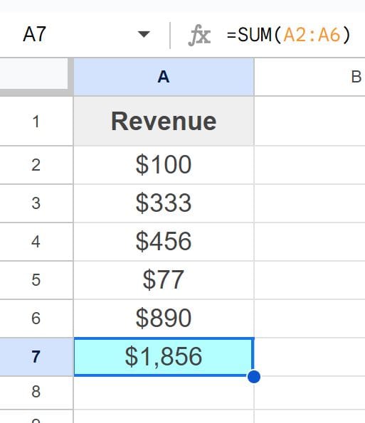
In the image below, you can see that the reference has been changed so that the SUM function is only summing rows 2 through 6, which allows the SUM function to correctly sum the numbers above it.
Corrected formula:
=SUM(A2:A6)
Personally I prefer to put my SUM function at the top of the sheet, so that any amount of data can be added below it without the formula getting in its own way.
When you are summing cells with formulas that have an error
If you are summing a column that contains formulas, if one of the formulas in the column you are summing displays an error, the SUM function will display the same error which can be confusing. This may cause you to think that there is an error with the SUM function, when it's actually an error with a formula contained within the range that you are trying to sum.
Make sure that all of the cells/formulas in the range that you are summing are calculating correctly.
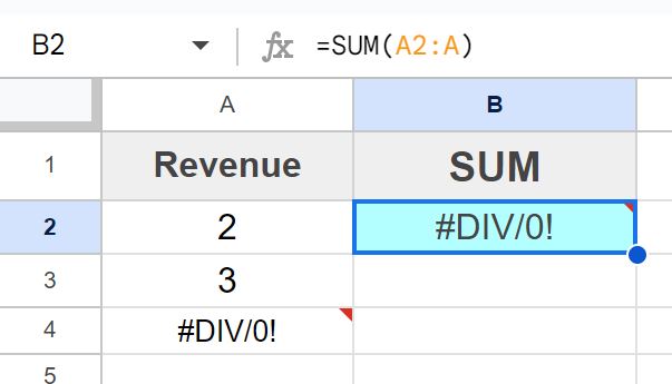
As you can see in the image below, cell A4 is displaying a divide by zero error: #DIV/0!
The SUM function in cell B2 is also displaying the same error, since the SUM function is referring to the range that the original error is in. To fix this, the formula in cell A4 must be fixed.
To fix the divide by zero error, make sure that your division formula is referring to the correct cells, and make sure that the data it is referring to is not missing. If the division formula is set up correctly and you simply want to make the error go away, use the IFERROR function to handle the error, like this: =IFERROR(G2/J2,0)
This will remove the error so that the SUM function can calculate the specified range.
=SUM(A2:A)
The formula in this example is entered correctly, but is displaying an error because one of the cells in the range that it's being summed has an error.
Hidden or filtered rows
If you have hidden rows in your spreadsheet, this can cause the SUM function to give a result that is not expected. The formula technically calculates correctly, but if you don't know the rows are hidden it can give a larger number than you expect by adding numbers that you cannot see.
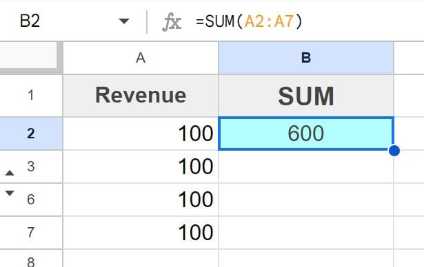
As you can see in the image below, rows 5 and 5 are hidden, and the SUM function is giving a total that is obviously more than the numbers displayed in column A add up to. This is because there are numbers in rows 4 and 5 that are being added by the function even though they are hidden.
=SUM(A2:A7)
The formula in this example is entered correctly, but is summing rows that are not displayed.
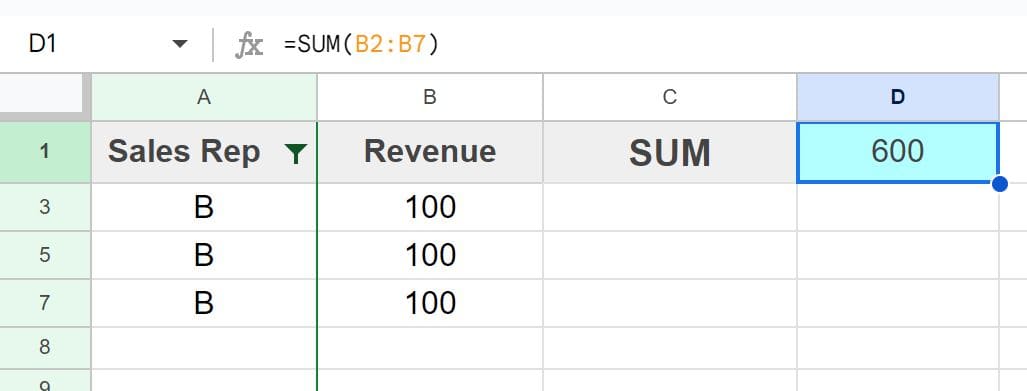
The same error can occur if you are using a filter in your spreadsheet. Notice that a filter is applied to column A and some of the rows have been filtered out, and just like in the example above the SUM function is showing a higher total than would be expected if you didn't know that the filtered rows were being summed as well.
=SUM(B2:B7)
The formula in this example is entered correctly, but is summing rows that are not displayed.
Now you know all of the different ways to fix the SUM function when it is not working correctly!