Using the UNIQUE function to remove duplicates in Google Sheets

The UNIQUE function is an incredibly useful function in Google Sheets, that can be used to remove duplicate entries, or in other words duplicate rows.

To remove duplicates with the UNIQUE function in Google Sheets, follow these steps:

1. Type "=UNIQUE(" or click “Insert” → “Function” → “Filter” → “UNIQUE”
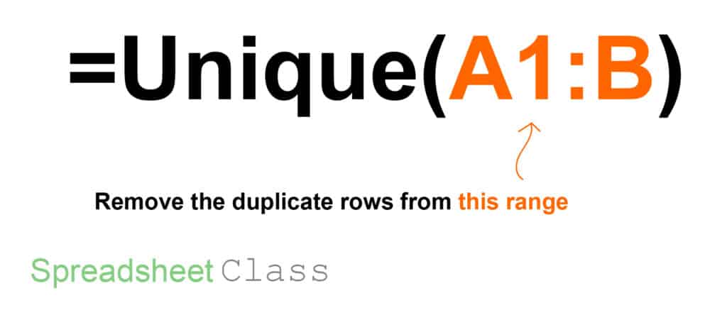
2. Type the range that contains the data you want to remove duplicates from, like this: A1:A15
3. Press "Enter" on the keyboard, and the duplicates will be removed. The formula will look like this: =UNIQUE(A1:A15)

This article focuses on using the UNIQUE function to remove duplicates, but you can also check out the lesson that goes over both methods to remove duplicates in Google Sheets.

Check out this lesson if you want to learn how to highlight duplicates instead of removing them.

Here are the Google Sheets UNIQUE formulas:

Remove duplicates from a single column

• =UNIQUE(A2:A)

Remove duplicates from multiple columns

• =UNIQUE(A3:B)

Sort unique entries

• =SORT(UNIQUE(A3:C))

Remove duplicates from another tab

• =UNIQUE(Sheet1!D3:D)

Remove duplicates horizontally

• =TRANSPOSE(UNIQUE(TRANSPOSE(B1:1)))

The Google Sheets UNIQUE formula:

The diagram below shows how the UNIQUE function works.

The Google Sheets UNIQUE function description:

Syntax:
UNIQUE(range)

Formula summary: “Returns unique rows in the provided source range, discarding duplicates. Rows are returned in the order in which they first appear in the source range.”

How to remove duplicates with the UNIQUE function

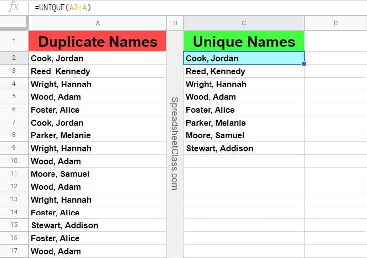
First let's start with a simple example, and remove the duplicates from a list of names that are in a single column.

The task: Remove the duplicate names

The logic: Use the UNIQUE function in column C to create a unique list of names, by referring to the list of names in column A

The formula: The formula below, is entered in the blue cell (C2), for this example

=UNIQUE(A2:A)

Using the UNIQUE function with a larger data set

Let's use a different example, where the original data that has duplicates in it, has multiple columns. We will start by referring to a single column, and then in the next examples we will actually refer to multiple columns.

But it will be beneficial to start with a single column, so that you can see how the result changes when you add more columns into the reference.

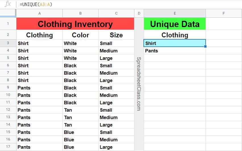
The image below shows a list of clothing items, the colors of the items, and the sizes of the items. Whether this data has duplicates or not, depends on how many columns are considered.

The task: Remove the duplicates from the list of clothing types (i.e. make a unique list of clothing types)

The logic: Use the UNIQUE function in column E, to remove the duplicates from the list of clothing types in column A

The formula: The formula below, is entered in the blue cell (E3), for this example

=UNIQUE(A3:A)

This content was originally created by Corey Bustos / SpreadsheetClass.com

Removing duplicates from multiple columns with the UNIQUE function

Now let's see what happens when you add an additional column into the formula's reference.

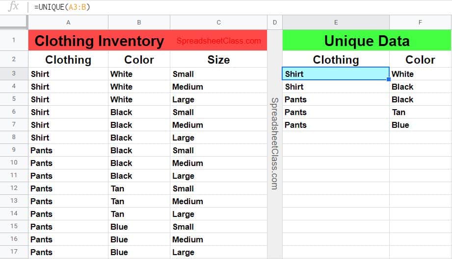
We will remove the duplicates while considering both the clothing "type" as well as the clothing " color. So both the type and the color must be the same to be considered a duplicate entry / row.

The task: Make a unique list of clothing type / color combinations

The logic: Use the UNIQUE function in column E to make a unique list of clothing types / colors by referring to columns A and B in the formula

The formula: The formula below, is entered in the blue cell (E3), for this example

=UNIQUE(A3:B)

Error checking (Part 1) with the UNIQUE function

Another handy thing that you can use the UNIQUE function for, is to check for errors in data.

Rather than intending to remove duplicates, we are going to use the UNIQUE function to make sure that there are no duplicates, by verifying that the list generated by the formula results is the same size (same number of rows) as the source data.

Let's say that someone wrote down all of the combinations of clothing types / colors / sizes that were found in inventory, and you want to make sure that they didn't record any duplicates.

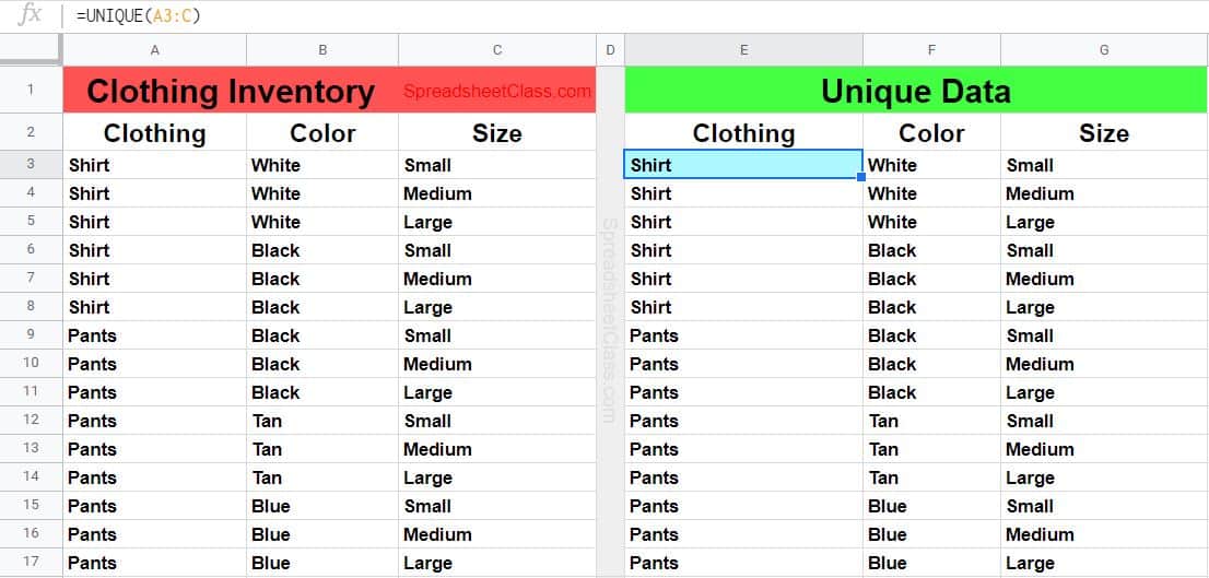
The image below shows what happens when another column is added to the reference, where the size is included in the formula reference, in addition to the type and the color.

As you can see, when this extra column is added, the results of the formula are the same as the source data, meaning that there were no duplicates to remove when considering all 3 columns.

So not only can you use the UNIQUE function to remove duplicates, you can also use it to verify that there are no duplicates.

The task: Verify that there are no duplicates in the data that shows clothing types, colors, and sizes

The logic: Use the UNIQUE function in column E, to create a unique list of entries from columns A through C

The formula: The formula below, is entered in the blue cell (E3), for this example

=UNIQUE(A3:C)

Creating a UNIQUE list of items

Let's go over another example of using the UNIQUE function with multiple columns.

One way that the UNIQUE function can be very helpful, is to find all of the different (unique) items in a long list of duplicates, such as from a sales report.

This is essentially the same as removing duplicate names from a list… but the difference is that in this case we have a very long list of items where we expect several duplicates due to repeated sales, and we are simply using the UNIQUE function to quickly give us a list of one of each item.

The functionality is the same as in the previous examples, but the purpose for using the function is different.

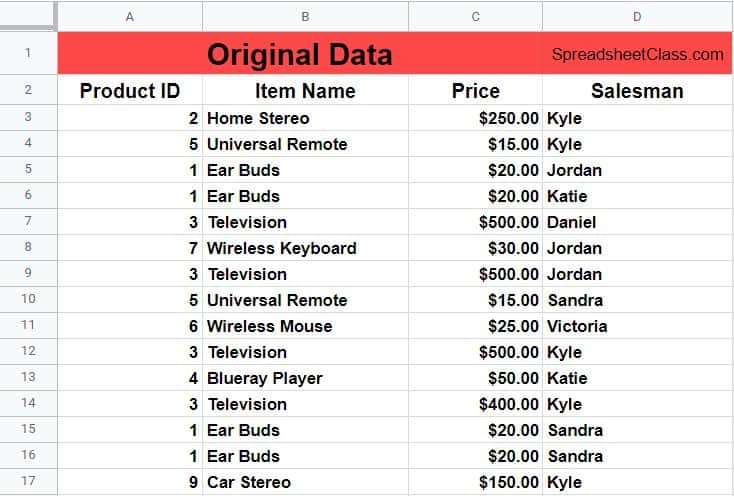
Below is a sales report that shows transactions that occurred. The sales data shows the "Product ID", the "Item Name", the price that the item was sold for, and the salesman who sold the item.

We are going to create a list of all the different types of items contained in the sales report by using the UNIQUE function.

The task: Create a list that shows one of each type of item (including product ID) from the sales report

The logic: In cell F3, refer to the range A3:B with the UNIQUE formula

The formula: The formula below, is entered in the blue cell (F3), for this example

=UNIQUE(A3:B)

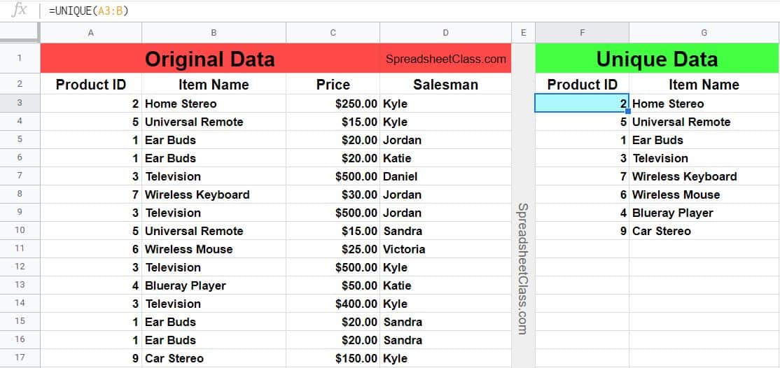
Now in columns F and G you can see a list of the different items contained in the sales report.

Error checking with the UNIQUE function

Here is another example of using the UNIQUE function to check errors in the data.

If you refer to multiple columns with the UNIQUE function, and you expect that the value in a single column should never be repeated, but you find that it is repeated… this will show you which value in the other columns is different and causing the extra entry to display.

In this example we are going to add the price column to the UNIQUE formula reference, and this will give us a list of all the different items and the prices that they were sold for.

In this case, let's pretend that the store which made these sales does not allow salesmen to give discounts, and soif the salesmen are following the rules there should not be any items sold for more than one price, and therefore there should never be more than one entry in the formula results that contains the same item name. We will demonstrate catching someone breaking this rule.

The task: Create a list of items (including the product IDs), and the price that the items were sold for

The logic: In cell F3, refer to the range A3:C with the UNIQUE formula

The formula: The formula below, is entered in the blue cell (F3), for this example

=UNIQUE(A3:C)

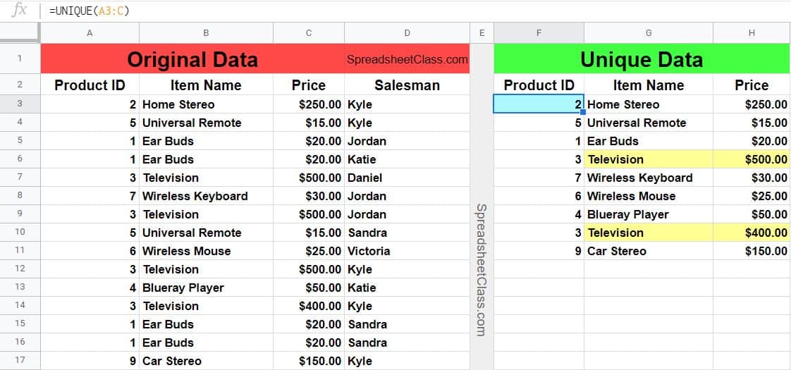
As you can see in the image above, there are two entries that contain the item name "Television". This is because someone sold a television for a discounted price, causing the UNIQUE function to see the change in column C, and therefore considering the entire entry / row a non-duplicate.

Sorting a unique list of entries with SORT and UNIQUE

You will likely find many times where you want to sort the list of unique entries that the UNIQUE function generates. You can do this by using the SORT function with the UNIQUE function, as demonstrated below.

In this case, sorting the list from the last example will help us more easily identify errors, by allowing you to see the item names sorted / grouped together.

The task: Sort a unique list of item names (including product ID), and the prices that they were sold for

The logic: In cell F3, refer to the range A3:C with the unique function, and then nest this function inside the SORT function

The formula: The formula below, is entered in the blue cell (F3), for this example

=SORT(UNIQUE(A3:C))

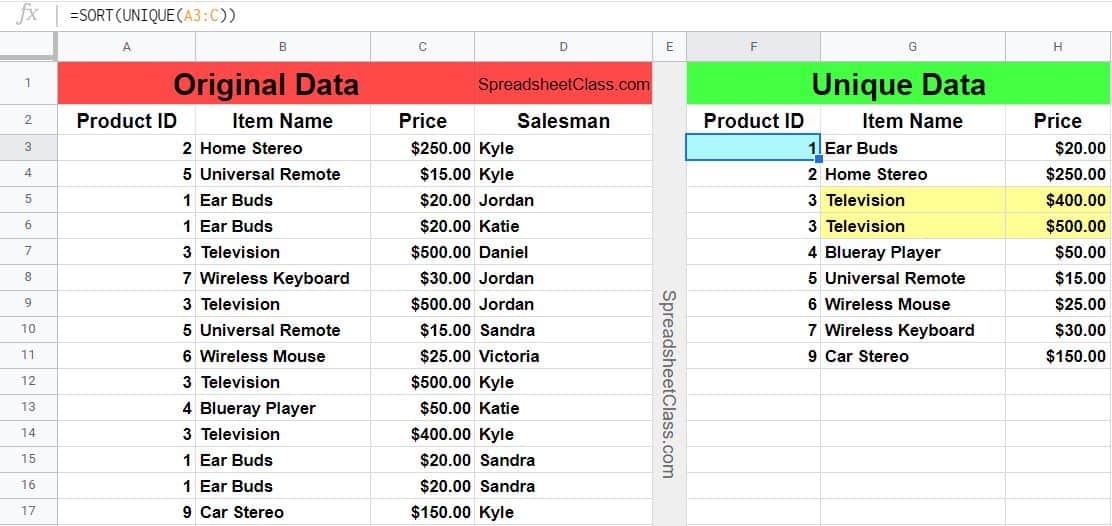
Now the data is sorted by item name / product ID, and the two entries that contain the item name "Television" are grouped together. This grouping / sorting makes it easier to identify errors, or in other words to identify entries that contain incorrect values in a certain column.

Note that we simply sorted by the first column (product ID), and so we didn't need to enter any criteria for the SORT function. But if we had wanted, we could have also specified the column to sort by and the order to sort by, like this:

=SORT(UNIQUE(A3:C),1,true)

Learn how to use the SORT function

Removing duplicates from another tab

You may find that you want to have your UNIQUE formula on a different tab than the data that it refers to, and so here is an example where we do exactly that.

When using the UNIQUE function to remove duplicates from another tab, in the formula reference include the name of the tab that you are referring to, followed by an exclamation point, like this =UNIQUE(Sheet1!D3:D).

But remember that if there is a space included anywhere in the tab name, you must include an apostrophe before and after the tab name, like this =UNIQUE('Sheet 1'!D3:D)

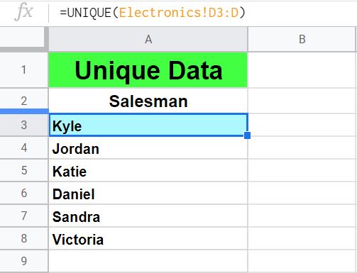
In the example below, the same raw data from the last example is held on the tab named "Electronics". We are going to put the UNIQUE function on a different tab, and create a unique list of salesmen found on the report.

The task: Create a unique list of salesmen from the data on the "Electronics" tab, and put the formula results on a different tab

The logic: Refer to the range A3:D from the "Electronics" tab with the UNIQUE function, where the function is held in another tab

The formula: The formula below, is entered in the blue cell (A3), for this example

=UNIQUE(Electronics!D3:D)

Formula tab:

=UNIQUE(Electronics!D3:D)

Removing duplicates horizontally

If you use the TRANSPOSE function, you can use the UNIQUE function to remove duplicates horizontally, or in other words to remove duplicate columns.

The TRANSPOSE function turns columns into rows, and rows into columns. It is needed to remove duplicates horizontally because the UNIQUE function only removes rows, and so to remove duplicates from the columns, you must first turn the columns into rows.

You must use the TRANSPOSE function twice when doing this.

First the TRANSPOSE function is applied to the source data to make it vertical. Then the UNIQUE function is applied, so that the duplicate rows are removed (Rows which were once columns). Then the TRANSPOSE function is applied again, to change the rows back into columns.

So in short, make the horizontal data vertical, use the UNIQUE function, and then switch it back again, as shown below.

The task: Remove the duplicate entries from row 1

The logic: Refer to row 1 with the TRANSPOSE function, then apply the UNIQUE function to the results of that, and then apply the TRANSPOSE function to the results of the other two functions.

Or in other words, nest the TRANSPOSE function inside of a UNIQUE function, and nest those two formulas inside another TRANSPOSE function.

The formula: The formula below, is entered in the blue cell (…), for this example

=TRANSPOSE(UNIQUE(TRANSPOSE(B1:1)))

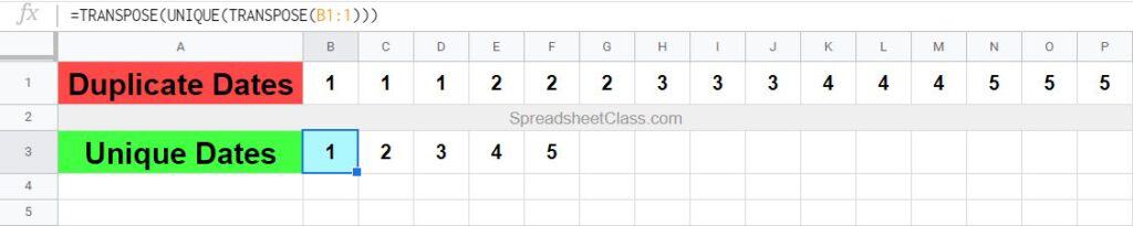
As you can see in the image above, the duplicate numbers were removed from row 1, and a horizontal, unique list of numbers is in row 3.

Pop Quiz: Test your knowledge

Answer the questions below about the UNIQUE formula, to refine your knowledge! Scroll to the very bottom to find the answers to the quiz.

Question #1

Which of the following formulas will remove duplicates from column A?

1. =UNIQUE(A1:B)
2. =UNIQUE(A1:A)
3. =UNIQUE(B1:B)

Question #2

Which of these formulas will remove duplicates from multiple columns?

1. =UNIQUE(A1:B)
2. =UNIQUE(A1:A)
3. =UNIQUE(B1:B)

Question #3

Which of the following formulas will remove duplicates horizontally?

1. =UNIQUE(B1:1)
2. =TRANSPOSE(B1:1)
3. =TRANSPOSE(UNIQUE(TRANSPOSE(B1:1)))

Question #4

Which of the following formulas will remove duplicates horizontally?

1. =UNIQUE(B1:1)
2. =TRANSPOSE(B1:1)
3. =TRANSPOSE(UNIQUE(TRANSPOSE(B1:1)))

Question #3

Which of the following formulas will remove duplicates horizontally?

1. =UNIQUE(B1:1)
2. =TRANSPOSE(B1:1)
3. =TRANSPOSE(UNIQUE(TRANSPOSE(B1:1)))

Question #4

True or false: The unique function removes duplicate rows?

1. True
2. False

Question #5

True or false: If you refer to the range A1:B with the unique function, the data in both columns A and B must be the same as the data in another row, to be considered a duplicate…. i.e. when comparing two rows, if the data is the same in column A but different in column B, the rows will not be considered duplicates.

1. True
2. False

Answers to the questions above:

Question 1:  2

Question 2:  1

Question 3:  3

Question 4:  1

Question 5:  1