ARRAYFORMULA & 5 ways to apply a formula to an entire column in Google Sheets

When using formulas in Google Sheets you will often need to apply a formula to an entire column, and there are several different ways that you can do this, and in this lesson I am going to teach you all of them. Personally my favorite method of applying a formula to an entire column is by using the ARRAYFORMULA function, but I will also show you several other easy methods.

Below are the two easiest ways to apply a formula to an entire column, and then further below we will go over the 5 methods in detail.

Later I will also show you how to use the click and drag method to autofill, but if you want to fill the entire column the shortcut is much faster.

The formula above will apply the functionality of the formula to the entire column, by using a single formula entered into a cell. This is exactly what the ARRAYFORMULA function does, and why it's so amazing.

For example, note the two IF formulas below. The first one is an ordinary IF formula that refers to a single cell, but the second formula uses the ARRAYFORMULA function, and is applied to the entire column.

=IF(A1=1,1,0)
=ARRAYFORMULA(IF(A1:A=1,1,0))

Click and drag fill handle method to apply a formula to an entire column

If you want, you can easily copy a formula into a range or a column by using the "fill handle".

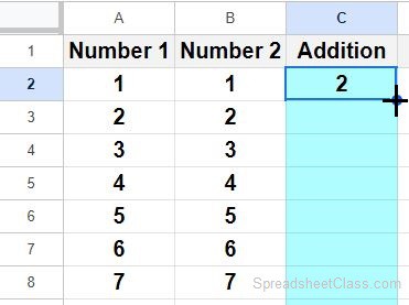
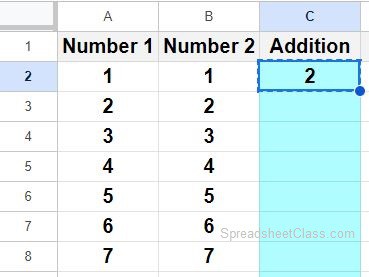
Simply click on the cell that contains the formula that you want to copy / fill down, hover your cursor at the bottom right corner of the cell (a plus sign / crosshairs will appear)… click your mouse, hold the click, and drag your cursor downwards until you have reached the row where you want you formula to be copied to, then release your click.

This will use the autofill feature to copy the formula at the top, into the column / the cells below. Google Sheets will automatically adjust the cell references for the appropriate row number when you use autofill or copy and paste formulas.

Fill down keyboard shortcut method to apply a formula to an entire column

Another way to use autofill is to use the keyboard shortcut "Ctrl" + "D" which fills down a formula to the bottom of the selected range. This is why we use another shortcut to quickly select an entire column. This makes it very fast to apply a formula to an entire column.

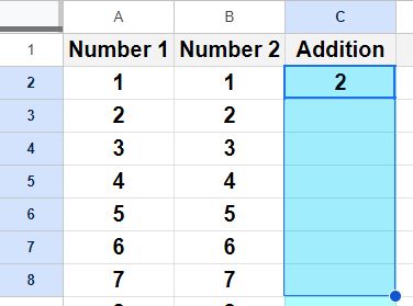
Simply select the cell that contains the formula you want to copy down, press "Ctrl" + "Shift" +the down arrow key on the keyboard, and this will select all of the cells to the bottom of the column (where the cell at the top of the selected range contains the formula to be copied).

The press "Ctrl" + "D" on the keyboard and Google Sheets will automatically copy / fill the formula at the top of the selected range, into the entire column / the entire range of selected cells.

Copy and paste method to apply a formula to an entire column

You can also copy and paste your formulas to apply them to an entire column.

Select the cell that contains the formula to be copied, press "Ctrl" + "C" on the keyboard to copy the cell

Then press "Ctrl" + "Shift" + the down arrow key on the keyboard to select all of the cells in the column

Press "Ctrl" + "V" to paste the formula / apply the formula to the entire column.

Using autofill and copying / pasting are essentially the same thing, just done in different ways.

Using the "Suggested autofill" feature to apply a formula to an entire column

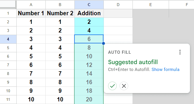
Another way that you can apply your formula to an entire column in Google Sheets, is to use the "Suggested autofill" prompt that will appear after you enter a new formula when there is more data in the rows below), as shown in the image below. It will show you a preview of the autofill results, and you can click the green checkmark to accept the autofill, or click the "X" to reject it. This is a really handy feature.

If you want more examples of how to use autofill and how to copy and paste formulas, check out this lesson on using “fill down” to copy formulas. Below we will go over using ARRAYFORMULA with several examples.

But now we will move on to using the ARRAYFORMULA function to apply a formula to an entire column, which has lots of different uses so I will show you many ways to use this very useful formula.

ARRAYFORMULA method to apply a formula to an entire column

The video above is the condensed version of the ARRAYFORMULA video lesson. Scroll down to the bottom of the page to see the extended version with more examples.

This article shows how to use ARRAYFORMULA in Google Sheets, but click here if you want to learn how to use arrays in Excel.

Here are the various ways to use the ARRAYFORMULA function:

Refer to a column

• =ARRAYFORMULA(A2:A)

Refer to a row

• =ARRAYFORMULA(B1:1)

Sum / Multiply columns

• =ARRAYFORMULA(A3:A+B3:B)
• =ARRAYFORMULA(A3:A*B3:B)

ARRAYFORMULA IF

• =ARRAYFORMULA(IF(B3:B>0.6,"Passing","Fail"))

Combine first and last name

• =ARRAYFORMULA(B3:B&", "&A3:A)

Sum entire tables of data

• =ARRAYFORMULA(A3:B+D3:E+G3:H)

Pulling data from another sheet

• =ARRAYFORMULA(List!A3:B)

ARRAYFORMULA shortcut:

If you prefer, you can simply type the ARRAYFORMULA function into the formula bar… or you can also use the keyboard shortcut to turn your formula into an "Array Formula".

After typing your formula (while your cursor is still in the formula bar), press the keys Ctrl + shift + enter, and this will wrap your formula in the ARRAYFORMULA function automatically.

For example, type =C1:C, and then press Ctrl + shift + enter, and your formula will turn into =ArrayFormula(C1:C).

Note that if you use the ARRAYFORMULA shortcut in a formula that has a reference to a single cell, Google Sheets may or may not change that cell reference into a range / column, so always make sure that your references are correct. The ARRAYFORMULA function only works on multiple cells if you are referring to a range of cells.

The Google Sheets ARRAYFORMULA function:

So before we get started with using the ARRAYFORMULA function in examples, let's go over what the function does.

Google Sheets description for the ARRAYFORMULA function:

Syntax:
ARRAYFORMULA(array_formula)

Formula summary: “Enables the display of values returned from an array formula into multiple rows and/or columns and the use of non-array functions with arrays”

Below are two diagrams that show how the ARRAYFORMULA  function works. You will find examples of these formulas further below.

ARRAYFORMULA Diagram 1

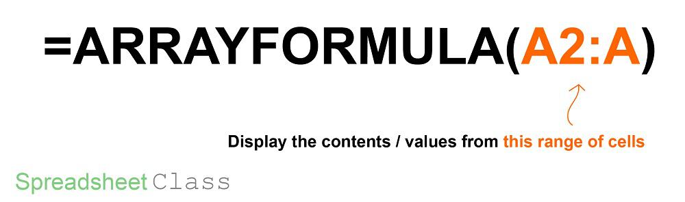
This diagram shows the most basic way of using ARRAYFORMULA, which is to refer to a range of cells.

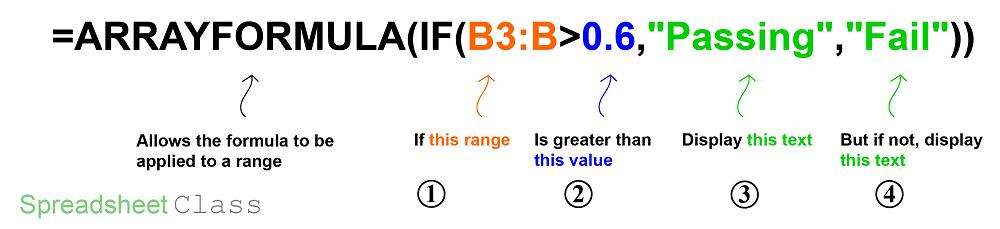
ARRAYFORMULA Diagram 2

This diagram shows how the ARRAYFORMULA function can be used to apply a formula to an entire column.

Get your FREE Google Sheets formula cheat sheet

Referring to a column with the ARRAYFORMULA function

One of the most common and basic ways to use the ARRAYFORMULA function, is all by itself without another formula being involved… to simply refer to a column or range of data with a single formula.

This is how we will use ARRAYFORMULA to begin with, but then after you get a good grasp on using the formula itself, we will move on to using ARRAYFORMULA to apply other formulas across ranges of cells.

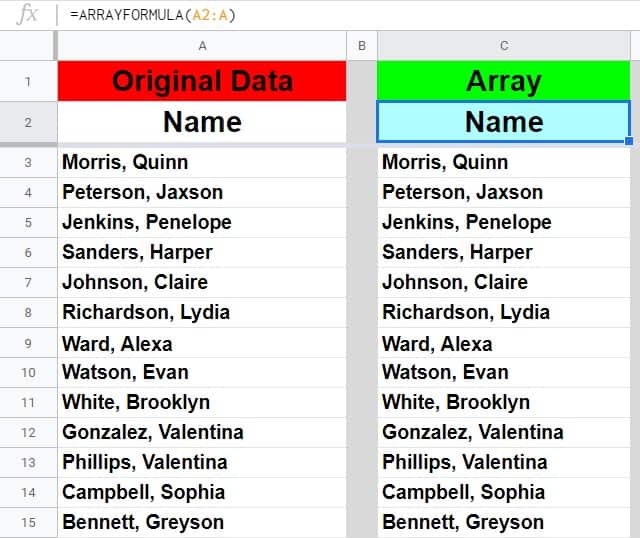
So in this example we will display a list of names from one column, in another column in the spreadsheet.

The task: Display a list of names in another column

The logic: In column C, refer to the list of names that are in column A with ARRAYFORMULA

The formula: The formula below, is entered in the blue cell (C2), for this example

=ARRAYFORMULA(A2:A)

Referring to a row with the ARRAYFORMULA function

It’s good to note that you can also use the ARRAYFORMULA function to refer to rows / horizontal ranges as well.

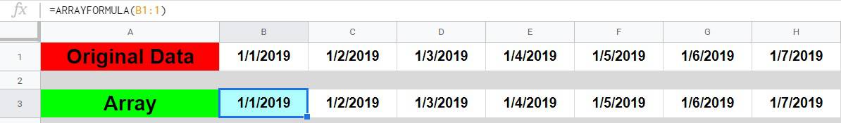
In this example we will refer to a row of cells that have dates in them, and display that list of dates in another row by using the ARRAYFORMULA function.

The task: Display a list of dates in another row

The logic: In row 3, refer to the list of dates that are in row 1 with ARRAYFORMULA

The formula: The formula below, is entered in the blue cell (B3), for this example

=ARRAYFORMULA(B1:1)

By SpreadsheetClass.com

How to SUM and multiply columns in Google Sheets

Now let's use ARRAYFORMULA to extend a formula in Google Sheets, so that it applies to an entire column.

You may often find the need to sum or multiply entire columns in Google Sheets, and if you want to achieve this with a single formula then using ARRAYFORMULA is the way to do it.

This example shows how to use ARRAYFORMULA to extend addition and multiplication formulas.

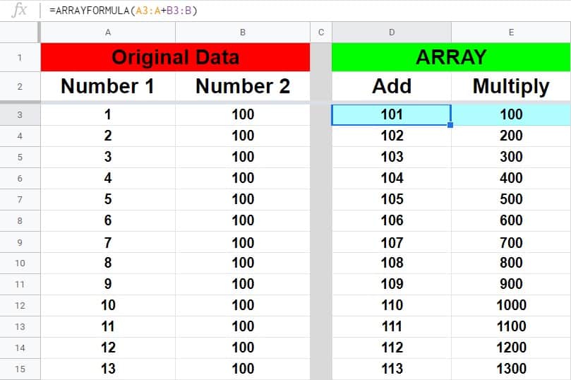
Columns A and B are lists of numbers… and columns D and E add/multiply these numbers by extending addition and multiplication formulas down the column with the ARRAYFORMULA function.

In column D, you can see that the addition formula in cell D3 extends its functionality downward into the cells below by using only a single formula, and you can see in column E that the multiplication formula does the same.

The task: Apply the addition and multiplication formulas to an entire column

The logic: Wrap the addition and multiplication formulas in the ARRAYFORMULA function, and specify an entire column as the range

Formula: The formulas below are entered initially into cells D3 and E3 (blue cells), for this example

=ARRAYFORMULA(A3:A+B3:B) is entered into cell D3

=ARRAYFORMULA(A3:A*B3:B) is entered into cell E3

Using ARRAYFORMULA to extend the IF function

Here is another example where we will apply a formula to an entire column in Google Sheets, but this time we will use the IF function.

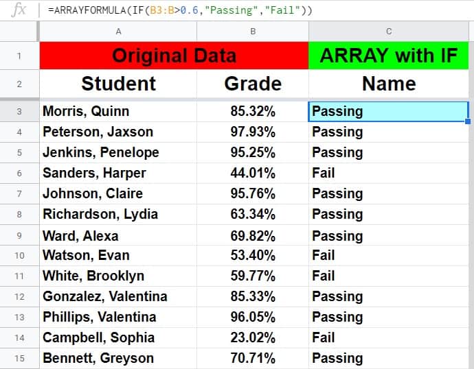
Let's say that you have an IF formula that you have setup to display whether a student is passing/failing based on their grade, and that you want to apply this formula to the entire column. We will do this by wrapping the IF formula in the ARRAYFORMULA function.

In the example image below, in columns A and B, is a list of student names and their grades. The formula in column C uses the IF function to display "Passing" if the student's grade is above 60% (0.6), and displays "Fail" if the grade is not above 60%. But the most important thing to note in this example, is that the IF function has been applied to the column by using the ARRAYFORMULA function.

The task: Apply the IF formula to an entire column

The logic: Wrap the IF formula in the ARRAYFORMULA function, and specify an entire column as the range

The formula: The formula below, is entered in the blue cell (C3), for this example

=ARRAYFORMULA(IF(B3:B>0.6,"Passing","Fail"))

How to combine first and last name with ARRAYFORMULA

Another very useful way that you can use ARRAYFORMULA, is to combine columns, such as when you need to combine first and last name into a single column.

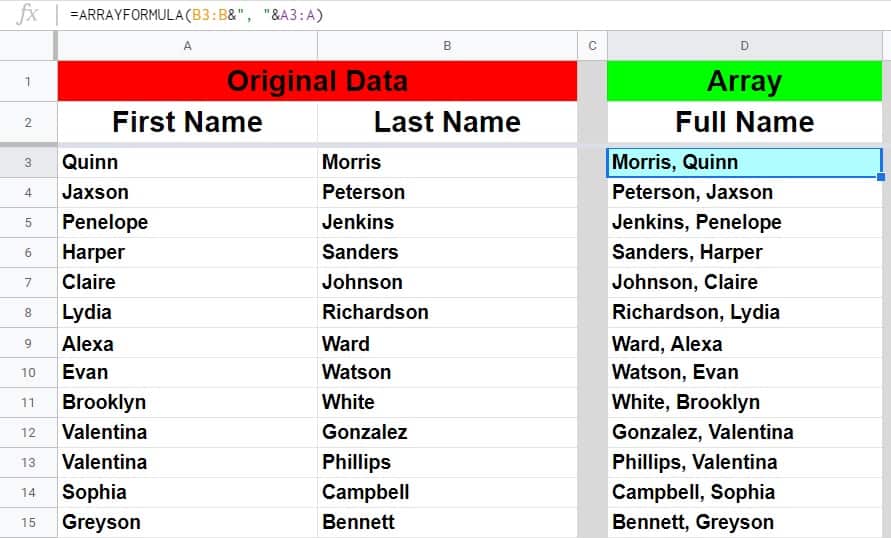
When using ARRAYFORMULA to combine cells/columns, you must use the "&" operator between each of the values/references that you specify (shown in the example).

In the example image below, column A has first names and column B has last names.

By using the ARRAYFORMULA function with the "&" operator, these names are combined in column D.

The task: Combine the first and last names into "Last, First" format

The logic: Horizontally combine columns A and B, with a comma and a space between them, by using the ARRAYFORMULA function and the "&" operator

The formula: The formula below, is entered in the blue cell (D3), for this example

=ARRAYFORMULA(B3:B&", "&A3:A)

How to sum entire tables of data with ARRAYFORMULA

Earlier I showed you how to sum columns of data with ARRAYFORMULA, but you can also use this function to sum data across entire tables of data.

When you add a range that has two or more columns/rows to another range of the same size, the ARRAYFORMULA function will sum each row/column across the ranges specified.

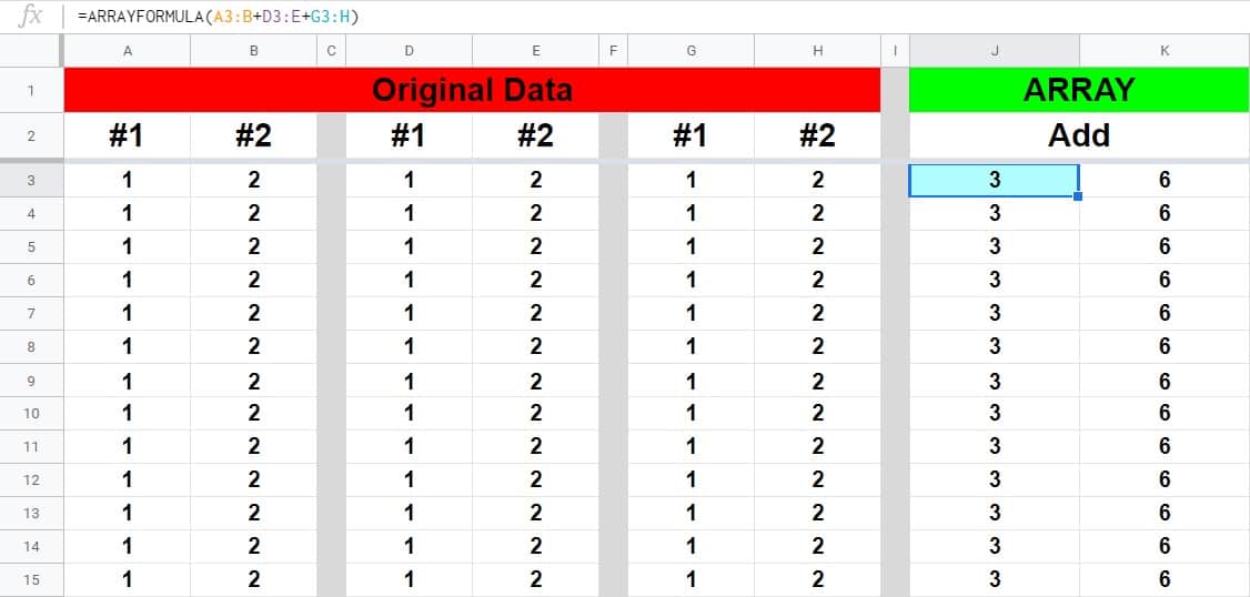
So as you'll see in the formula below, there are three different two-column tables that are being added together with the ARRAYFORMULA function. The first column of the first range is added to the first column of the second range and then added to the first column of the third range. The function does the same for the second column as well, or for any number of columns as long as the range you are adding are the same size.

This can be visualized as stacking the tables on top of each other and then summing the stacked/overlapping numbers.

The task: Sum the values from three different tables, where each column from each table is added to the same column from the other tables

The logic: Use the ARRAYFORMULA function to sum the columns from three different two-column ranges, where the first columns are added with the other first columns, and the second columns are added with the other second columns

The formula: The formula below, is entered in the blue cell (J3), for this example

=ARRAYFORMULA(A3:B+D3:E+G3:H)

This content was originally created and written by SpreadsheetClass.com

Pull data from another sheet with ARRAYFORMULA

A very common situation that requires the use of the ARRAYFORMULA function, is when you need to pull data from another sheet (tab) in Google Sheets. Earlier we went over how to simply refer to a range of data by using the ARRAYFORMULA function within the same tab, and you can use this same method to refer to data in another tab as long as you specify the tab name that you are pulling the data from, when typing the reference into the formula.

In this example we will cover two important things. The first, is that you can use ARRAYFORMULA to refer to data on other tabs, and the second is that you can use ARRAYFORMULA to refer to the entire range of data with multiple rows and columns.

In this example we have a list of first and last names on one tab, that we want to display in another tab. To do this follow the example below.

As with most formulas, when using ARRAYFORMULA to refer to data from another tab, type the name of the tab that you are pulling from, followed by an exclamation point, followed by the row/column reference.

Remember that if your tab name has a space in it, you must type apostrophes before and after the tab name (Example: 'Tab Name'!A3:B). However in this example the tab name that we will use is named "List", and so we don't need apostrophes.

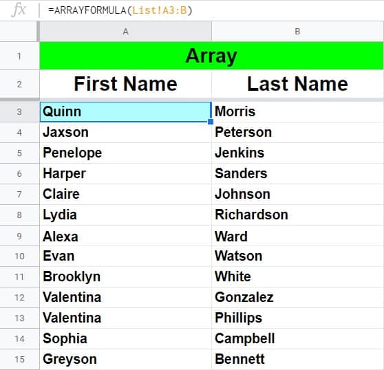
The task: Display the data that is in columns A and B from the tab that is named "List", in columns A and B in a new/different tab

The logic: In a new tab, display the data from columns A and B from the "List" tab, by referring to the data with the ARRAYFORMULA function

The formula: The formula below, is entered in the blue cell (A3), for this example

=ARRAYFORMULA(List!A3:B)

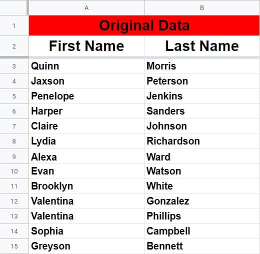
Source data from "List" tab:

Separate tab displaying referenced data/array:

Pop Quiz: Test your knowledge

Answer the questions below about the ARRAYFORMULA function, to refine your knowledge! Scroll to the very bottom to find the answers to the quiz.

Classroom downloads:

ARRAYFORMULA function cheat sheet (PDF)

Complete Google Sheets formula cheat sheet

Click the green "Print" button below to print this entire article.

Question #1

Which of the following formulas refers to a column of data?

1. =ARRAYFORMULA(A12:12)
2. =ARRAYFORMULA(G:G)
3. =B1

Question #2

Which of the following formulas refers to a row of data?

1. =J3
2. =ARRAYFORMULA(U1:U)
3. =ARRAYFORMULA(9:9)

Question #3

True or False: The following formula will not apply to an entire column, because it is not wrapped in the ARRAYFORMULA function:

=IF(D:D=100,"Perfect","Not Perfect")

1. True
2. False

Question #4

Which of the following formulas refers to a range in another sheet?

1. =ARRAYFORMULA(A1:Z)
2. =ARRAYFORMULA(Values!A3:B)

Question #5

Which of the following formulas refer to a range with multiple columns? (Select all that apply)

1. =ARRAYFORMULA(Values!A:B)
2. =ARRAYFORMULA(A:A)
3. =ARRAYFORMULA(C:B)
4. =ARRAYFORMULA(List!G:G)
5. =ARRAYFORMULA(Y:Z)

Question #6

Which of the following formulas will apply a multiplication formula to an entire column?

1. =ARRAYFORMULA(A3:AxB3:B)
2. =A3:A*B3:B
3. =ARRAYFORMULA(A3:A*B3:B)
4. =A3:AxB3:B

Answers to the questions above:

Question 1: 2

Question 2: 3

Question 3: 1

Question 4: 2

Question 5: 1, 3, 5

Question 6: 3

The video below is the extended version of the ARRAYFORMULA video lesson, with more examples included.