
In Google Sheets you can easily apply strikethrough to your cells / text. Strikethrough is a useful formatting option when you want to visually indicate that certain information is no longer relevant or should be crossed out. It's a simple yet effective way to convey changes or updates in your data.
In this lesson I am going to show you three different ways to apply strikethrough in your Google spreadsheet. I will also show you how to apply strikethrough to specific words in the cell.
To apply strikethrough to text in Google Sheets, select the cells that contain the text that you want to apply strikethrough to, and then click the strikethrough button on the top toolbar (looks like an S with a line through it).
To use strikethrough in Google Sheets with the keyboard shortcut, follow these steps:
- Select the cell or cells that you want to apply strikethrough to
- Press Alt + Shift + 5 (For Windows). For Mac, press Command + Shift + X
After following the steps above, the selected text or cell will have strikethrough formatting applied.
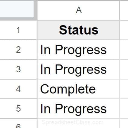
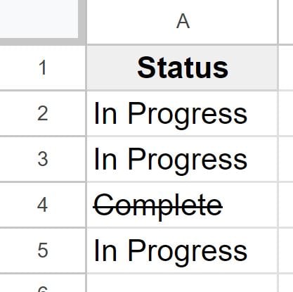
The image above shows data before strikethrough was applied, and the image below shows what it looks like after strikethrough has been applied to a cell.
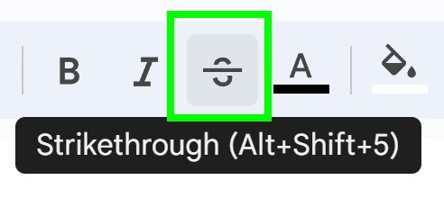
Method 1: Click the "Strikethrough" button on the top toolbar
The way that I prefer to apply strikethrough in Google Sheets, is to Simply click the button on the top toolbar.
As you can see in the image below, the strikethrough button is the letter S with a line drawn through it. It is right beside the button for text color and italic font. When you hover your cursor over the button, it will say "Strikethrough" and will also show you the keyboard shortcut.
To use this method, simply select the cells that you want to apply strikethrough to, then click the button on the top toolbar.
Method 2: Use the keyboard shortcut to apply strikethrough
Applying strikethrough to text in Google Sheets can also be done easily by using a keyboard shortcut.
Underline shortcuts for Google Sheets:
For Windows: Alt + Shift + 5
For Mac: Command + Shift + X
To use strikethrough with the keyboard shortcut in Google Sheets, select the text / cells that you want to apply strikethrough formatting to, then press Alt + Shift + 5 (For Windows) or Command + Shift + X (For Mac).
Following these steps, you'll see the selected text or cell with strikethrough formatting applied.
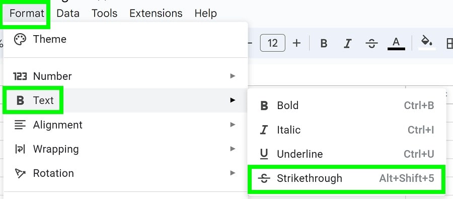
Method 3: Use the "Format" menu to apply strikethrough
In this section, we'll go over how to apply strikethrough formatting to text within Google Sheets using the "Format" menu.
To use strikethrough in Google Sheets, follow these steps:
- Select the cell(s) that contain that text that you want to apply strikethrough to
- Click "Format" on the top toolbar
- Click "Text"
- Click " Strikethrough"
Once you've completed these steps, the selected text will appear with a strikethrough line, indicating that it has been crossed out. This can be particularly handy when you want to show changes or deletions in your spreadsheet.
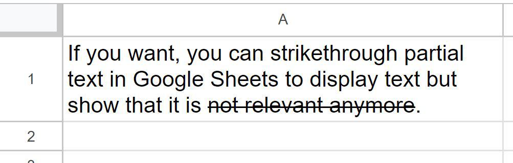
Strikethrough partial text & specific words in a cell
If you want, you can actually strike through a portion of the text in a cell instead of all of the text in the cell. I had been using Google Sheets for a long time and only recently discovered this.
To apply strikethrough to specific words or parts of text in a cell using a keyboard shortcut, follow these steps:
- Select the cells that contains the text you want to apply strikethrough to
- Double-click on the cell to enter edit mode
- Highlight the specific words or portions of text you want to apply strikethrough to
- Press Alt + Shift + 5 (For Windows) or Command + Shift + X (For Mac) on your keyboard
- Press Enter / Return on the keyboard
By following these steps, you can easily strike through only the selected words or portions of text within a cell, allowing you to format specific words without affecting the entire cell's content.
In the image below you can see that some of the text in cell A1 has strikethrough formatting, and some of it does not.
Note that any of the three methods that we went over in this lesson will also work for applying strikethrough to a portion of the cell's text (such as the "Format" menu method or the button on the top toolbar). Simply select the text that you want to format, and use any of the methods.
Removing strikethrough format
You may want to remove the strikethrough format, and this is done by using the same method as enabling strikethrough.
To remove strikethrough format in Google Sheets, select the cell or cells that you want to remove strikethrough formatting from, then press Alt + Shift + 5 on the keyboard (Command + Shift + X for Mac), or click "Format" > "Text" > "Strikethrough".