

Understanding how to calculate percentage increase in a set of values is crucial for assessing growth or change over time, whether you’re tracking financial growth, project milestones, or any other numerical trends.
To calculate the percentage increase/decrease, first you subtract the initial value from the final value to find the difference, and then you divide that number by the initial value. =(Final-Initial)/Initial
To calculate percentage increase in Google Sheets, follow these steps:
- Enter the initial value in one cell, and enter the final value in another cell
- Subtract the initial value from the final value to determine the numerical increase/decrease
- Divide the numerical increase/decrease by the initial value. The final formula will look like this, where cell B2 is the final value and cell A2 is the initial value: =(B2-A2)/A2
- Format the cell containing the percentage increase as a percentage if it does not automatically display as a percentage (Select the cell, and click “Format as percent” (%) on the top toolbar)
After following the steps above, you will have successfully calculated the percentage increase between two values in Google Sheets.
This article focuses on calculating the increase in percentage from one number to another… but if you want you can click here to learn how to calculate the percentage of a total.
Now let’s go over some detailed examples of how to calculate percentage increase in Google Sheets.
Calculating percentage increase from one number to another
Let’s go over a basic example of calculating the percentage increase from one number to another.
Let’s say that in your spreadsheet, you have initial data in cell A2 (100) and final / new data in cell B2 (150). What we are going to do is calculate the percentage increase from 100 to 150. To do this, we will subtract 150 (cell B2) from 100 (cell A2), and then divide the result by 100 (cell A2). The final formula will be: =(B2-A2)/A2.
Notice how we used parenthesis to separate the subtraction portion of the formula, so that the spreadsheet calculates in the order that we want it to.
=(B2-A2)/A2
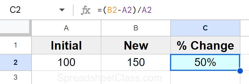
As you can see in the image above, cell C2 displays the calculated percentage increase (50%). This means that the number 150 is 50% more than the number 100, or in other words there was a 50% increase from the initial value to the new / final value.
Calculating the difference in an individual cell
If you want, instead of combining the subtraction problem and the division problem into one formula, you can use a cell that is designated for subtracting the initial value from the final value, and then you can refer to that cell in the division formula that is entered into a different cell.
In this example we have the initial value in cell A2, the new/final value in cell B2, then we are calculating the difference between the final value and the initial value in cell C2 with a simple subtraction formula, and then in cell D2 We Are calculating the percentage change by dividing the difference (Cell C2) by the initial value (cell A2). So cell C2 subtracts cell A2 from cell B2, and then we divide cell C2 by cell A2.
Cell C2 formula:
=B2-A2
Cell D2 formula:
=C2/A2
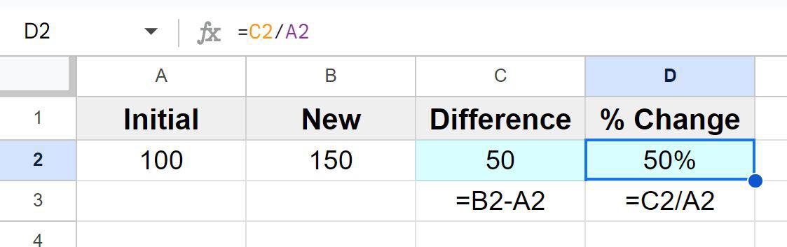
As you can see in the image above, cell C2 shows that the difference between the final value (cell B2) and the initial value (cell A2) is 50. Then cell D2 shows that the the result of the subtraction problem (cell C2) divided by the initial value (cell A2) is 50%, meaning that the percentage increase from the initial value to the final value was 50%.
Calculating percentage decrease
Calculating the percentage decrease is exactly the same as it is for calculating the percentage increase. To show you this, I am going to use the same exact setup from the previous example, and the only things that I am going to change is the initial value and final value (the difference between the two will be a negative number this time).
Again, set up your formula in the exact same way as you would when calculating percentage increase. Do not change the order of the cells that you subtract. When there is a percentage decrease between the initial value and the final value, there will also be a negative number when you find the difference between them (Initial – Final).
So in this example we have an initial number of 150 in cell A2, a final number of 100 in cell B2, and cell C2 uses the following formula to calculate the percentage decrease from cell A2 to cell B2: =(B2-A2)/A2
=(B2-A2)/A2
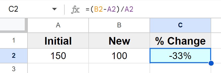
As you can see in the image above, cell C2 shows that the percentage decrease from cell A2 to cell B2 was -33%.
Calculate percentage increase from row to row / cell to cell
Sometimes you will have a sequence of numbers where you want to calculate the percentage increase/decrease from row to row, or column to column. This can be done easily with a formula.
To do this we use the same type of formula as in the previous example, but our initial value refers to the data in the previous row / column, and the final value refers to the data in the current row / column. Each time the formula is copied down the column (or through the row), the cell references increment 1 row / column as desired, and the calculation correctly refers to each preceding / succeeding cell as desired. This will be more clear when you see the example below.
To calculate percentage increase from cell to cell in rows or columns, follow these steps:
- Subtract the value in the preceding cell (initial value) from the value in the succeeding cell (final value)
- Divide the result by the value in the preceding cell (initial value)
- Format the cell(s) as “Percent”: Select the cells and then click the “Format as percent” button on the top toolbar
We are essentially telling Google Sheets to subtract the value in the previous row/column from the value in the current row/column, and then to divide the result / difference by the initial value (value from the previous row / column).
The formula in each row will display the percentage increase between the previous row and the current row.
In this example, we have a list of numbers in column A. What we are going to do is calculate the percentage increase from one row to the next. To do this, we use the following formula: =(A3-A2)/A2. This formula starts in cell B3 and is copied down the column.
The formula does not begin in cell B2, because row 2 is where the first data point is, and there is not a previous data point that we can compare for percentage increase.
=(A3-A2)/A2
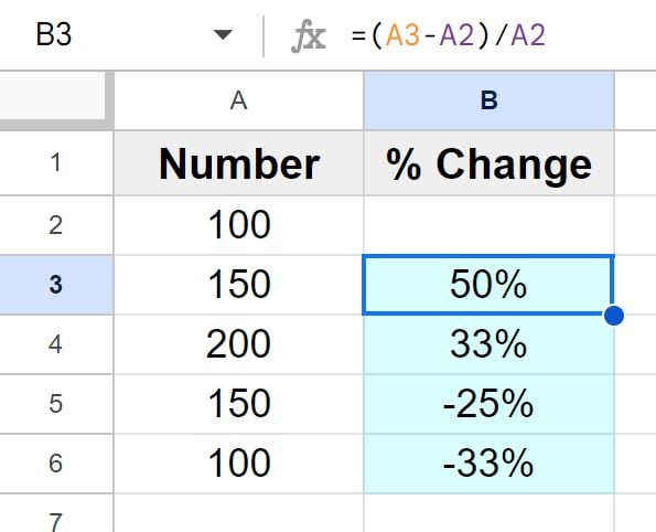
As you can see in the image above, cell B3 displays that there was a 50% increase from cell A2 (100) to cell A3 (150). The formula was copied down the column, and Google Sheets automatically adjusts the cell references, as shown below.
Cell B4 will have the formula: =(A4-A3)/A3
Cell B5 will have the formula: =(A5-A4)/A4
Cell B6 will have the formula: =(A6-A5)/A5
Let’s break down how the formula is working. First the formula subtracts cell A2 (Final value) from cell A3 (initial value). Then that result is divided by cell A2 (initial value).
Here is the logic of the formula in a way that is easy to understand:
=(Final-Initial)/Initial
=(Current row-Previous row)/Previous row
=(A3-A2)/A2
Calculate percentage increase from a fixed starting point
This example is going to be very similar to the last example, except in this case we are going to calculate the percentage increase from row to row by using a fixed starting point as the initial value. So we will calculate the percentage increase / decrease between the fixed starting point, and the data in each row.
In cell B3 we will calculate the percentage increase that took place from cell A2 to cell A3.
In cell B4 we will calculate the percentage increase that took place from cell A2 to cell A4.
In cell B5 we will calculate the percentage increase that took place from cell A2 to cell A5.
In cell B6 we will calculate the percentage increase that took place from cell A2 to cell A6.
Notice how the reference to cell A2 stays consistent as the formula is copied into the cells below (because it is our fixed starting point), but the other cell references increment one row each time the formula is copied, just like we want, so that each data point in each row can be compared to the fixed to starting point.
To make it so that the cell reference to the initial value / fixed starting point does not change when the formula is copied into other cells, we will put a dollar sign before the row reference, like this: A$2. This prevents the row reference from changing.
This same method works for copying formulas horizontally into other columns. In that case you would use a reference like this $A2 to prevent the column reference from changing. So when you want to prevent the column reference from changing when you copy the formula, put the dollar sign ($) before the column letter, and when you want to prevent the row reference from changing when you copy formulas, put the dollar sign before the row number.
=(A3-A$2)/A$2
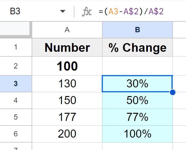
In the example image above, you can see that the number 100 is entered into cell A2, and this number is in bold font because it is going to be used as the fixed starting point. There are other numbers entered in column A, below cell A2. We want to find the percentage change for each of these numbers, in comparison to the initial fixed starting point at cell A2.
By using the following formula (starting in cell B3) we calculate the percentage increase that took place from cell A2 to cell A3: =(A3-A$2)/A$2
The special thing about the formula is what happens when it is copied into the cells below. When we copy the formula (in cell B3) into cell B4, the formula will adjust so that the initial value / reference to cell A2 remains the same, while the row reference to cell A3 will increment by 1 row, as desired.
Cell B4 will have the formula: =(A4-A$2)/A$2
Cell B5 will have the formula: =(A5-A$2)/A$2
Cell B6 will have the formula: =(A6-A$2)/A$2
The formula calculates the percentage between the fixed starting point, and each data point / each row.
Calculating from column to column instead of row to row
You can use this same method for columns instead of rows, as mentioned above. To do this, copy your formula to the right, and refer to the fixed starting point on the left side of your sheet. Your formula will look like the following, where the initial value is in cell A2, and the final / new value is in cell B2: =(B2-$A2)/$A2
Again, notice that when you copy the formula to the right instead of down, the dollar sign goes before the column letter of the cell address for the fixed starting point, so that when you copy your formula to the right, the column reference for the fixed point will not change.
Now you know how to calculate percentage increase in Google Sheets!