

After creating a chart, you can edit the “Data range” (the range that contains the data for the chart) at any time. In this lesson I will teach you how to change the data range for the chart, and how to make sure that the data actually appears on the chart.
To edit the data range on a chart in Google Sheets, follow these steps:
- Click on the chart that you want to edit, then click the 3 dots in the upper-right corner of the chart, then click “Edit chart” (You can also double-click on the chart to open the chart editor)
- On the “Setup” tab, in the “Data range” field, type the range that contains the data you want your chart to include (You can also click on the grid icon to select the range instead of typing it)
- If the new data range that is entered contains more columns of data than the original range that was entered, you will have to click “Add series” to add the new data to the chart.
Check out this lesson to learn more about adding a new series to a chart. But we will also go over that in more detail in this lesson.
Click here to learn how to create / customize charts in general.
Editing the chart data range (Removing data)
In this example, we have a chart that has two series (columns B and C). We are going to edit the data range to remove some of the data / remove column C.
To do this, simply double-click on the chart to open the chart editor, and on the “Setup” tab, enter the new data range in the “Data range” field.
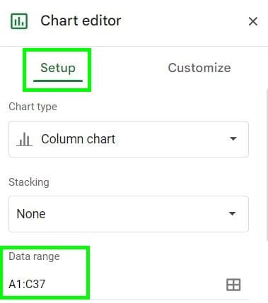
Notice that in this example the data range is initially A1:C37.
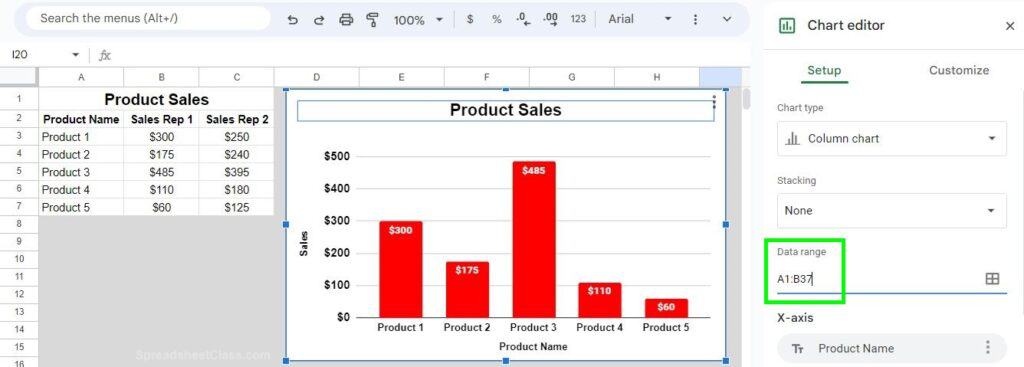
Change this range to A1:B37. This will remove column C from the chart.
As you can see in the image below, now the chart only displays the data for “Sales rep 1” and the second sales rep (data in column C) no longer displays on the chart.
When we edit the data range and the new range is smaller / data is removed, Google Sheets will automatically remove the data / series from the chart since the data that is being referred to no longer contains the series / data that was there before.
How to select the data range instead of typing it
If you want, instead of typing the desired data range into the “Data range” field, you can select the data range.
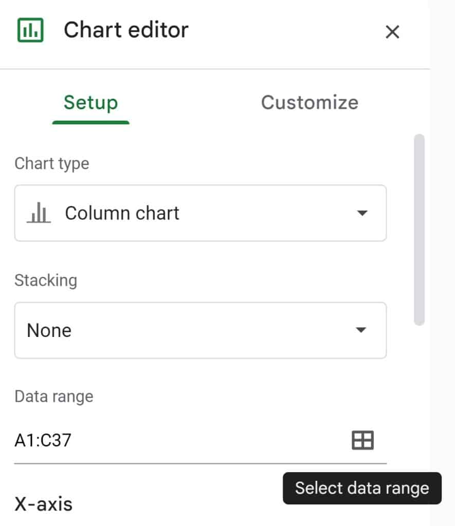
To do this, open the chart editor, and on the “Setup” tab, in the “Data range” field, click the grid icon that says “Select data range” when you hover your cursor over it. A menu will pop up, and you can then select the range of cells that contains the data you want your chart to display, and Google Sheets will automatically fill in the “Data range” field based on your selection.
This content was originally created by Corey Bustos / SpreadsheetClass.com
Editing the chart data range (Adding a series)
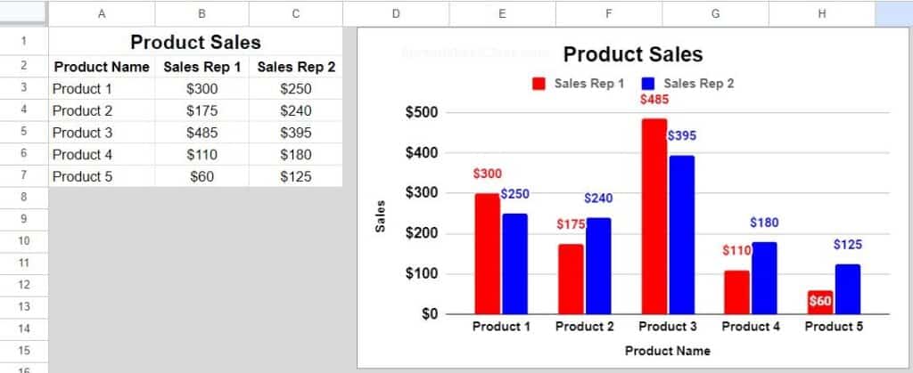
In this example we will edit the data range on the chart, but this time we will add data to the chart / the new range will contain more columns / data than the original range that was entered. When you edit the data range and add new data to the chart, you will need to manually add a new series to the chart.
A we are going to add sales rep 2 to the chart, by editing the data range and then adding a new series.
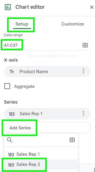
Double-click on the chart to open the chart editor. On the “setup” tab, enter the new data range in the “Data range” field (A1:C37)
Click “Add series”, and select the series to add (Sales rep 2 in this example)
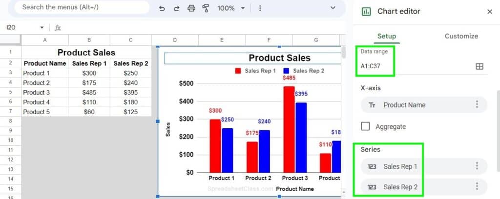
After following the steps above, the new data / new series will be added to the chart, as shown in the image below. Notice that the new data / series was added to the chart, and the new series is displayed in the chart editor.
Click here to get your free Google Sheets cheat sheet
How to edit the data range to chart data from another sheet
If you want, you can edit the data range so that you can display data on a chart that is on another sheet.
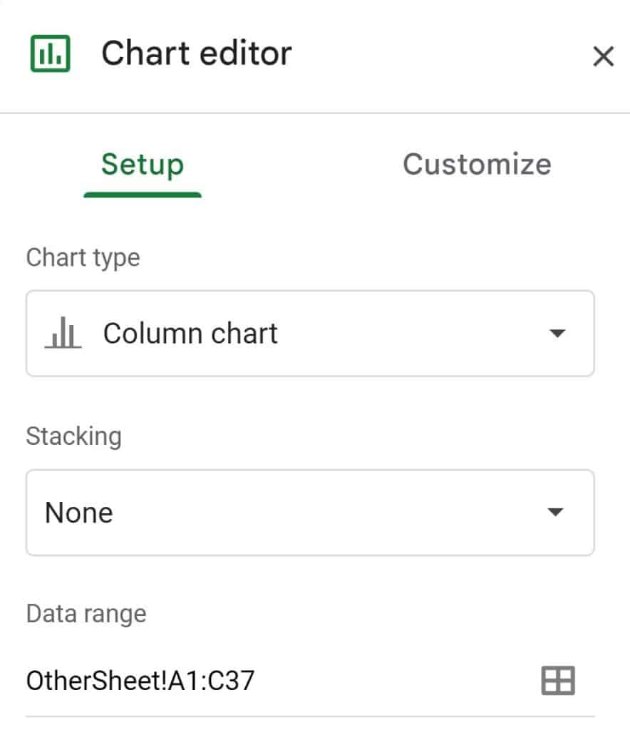
To do this, simply include the tab name in the data range, with an exclamation point between the tab name and the data range, as shown below.
So if we wanted to connect our chart to data on another sheet that is named “OtherSheet”, we would enter this in the “Data range” field: OtherSheet!A1:C37
Now the chart will display the data from the tab named “OtherSheet” where the chart is on a completely separate tab than the data.
Note that if the tab name has a space in it, you must put an apostrophe before and after the tab name, like this:
‘Other Sheet’!A1:C37
Now you know how to edit the data range of charts in Google Sheets, and you know how to make sure that the data is actually added to the chart after editing the data range.